The sequential probability ratio test, or SPRT, can be used as an efficient tool for process tolerance and mean shift determinations. It also provides for simplifying insights into the nature of random mean shifts when process tolerances and Type I/II errors are selected. The cumulative sum design of the test naturally compensates for random errors, and one-sided random shifts easily calculate as one-half of the process tolerance T, corresponding to a worst case error of ½ (a=b=.5). For a selected tolerance of 3 sigma, a long-term 1.5 sigma shift is simply the critical mean asymptotic limit of an indeterminate process for both one-sided and two-sided SPRTs.

Sequential Analysis Theory

Sequential analysis was created by Abraham Wald in 1943 for wartime military equipment development and inspections. Numerous examples of the theory’s practical applications and sampling economies were later published by Columbia University and example table exhibits of the 50 percent sampling economy can be found in the document. The bases are the probability inequality ratios that define the three inspection regions shown in Table 1 below.

Table 1
Accept H0	Continue to Inspect	Accept H1
I: P1N / P0N<b/ (1 – a)	II: b / (1 – a) < P1N / P0N < (1 -b) /a	III: P1N / P0N> (1 -b) /a

 

Where P_0N, P_1N are the probability density functions corresponding to the test H₀ and alternate H₁ hypothesis for the sequential set of observations X₁…X_N and a, b are the selected Type I (producer’s risk) and Type II (consumer’s risk) errors. The test is continued when inequalityratio (II) applies, and discontinued at the firstoccurrence of the ratios (I) or (III) resulting in the acceptance of hypotheses H₀ or H₁, respectively. When deployed during test applications for such popularprobability functions as the Binomial, Poisson and Normal distributions, the probability inequality ratios are usually transformed into the simple straight line forms Y₀ = S N + h₀, Y₁ = S N + h₁, where S is the common slope, N the sample number, and h₀, h₁ are the intercepts of the acceptance and rejection lines which delineate the regions. The cumulative sums S X_N of the observations are then compared with the straight line values for decision purposes. The concept is summarized in Table 2.

Table 2
Accept H0	Continue to Inspect	Accept H1
I: S XN < S N + h0	II: S N + h0 < S XN < S N + h1	III: S XN > S N + h1

One-Sided SPRT Process Mean and Shift Tests

As an example of the test’s applicability to mean testing, consider the sequence of observations X₁…X_N from a normally distributed population with a known standard deviation and unknown mean M.When the probability density ratios for the test hypotheses H₀: M = M₀, H₁: M = M₁ are inserted in Continue to Inspect test region of Table 1, thecumulativesum inequality (1) results. And upon inspection it is easily reduced to the straight line form (2).

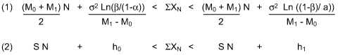
Dividing (1) by the cumulative sample size N transforms the Continue to Inspect region into the conceptually useful hyperbolic form:

Where Xca = 1 / N, SX_N is the cumulative average and Mc = (M₀ + M₁) / 2 is the critical mean and asymptotic limit for the test; i.e., cumulative averages Xca converge to Mc when N becomes sufficiently large and both h₀ / N, h₁ / N ? 0. The limit also occurs at the test’s maximum level of uncertainty or worst case error (a = b = ½) since h₀ / N = h₁ / N = 0 at these values. However, Wald has shown that all sequential tests eventually terminate with a probability of one which is evident by the geometry of the cumulative average test illustrated in the graph in Figure 1. Group size 4 random data from Shewhart’s normal bowl with the known average of 30 and standard deviation of 10 together with the Type I and Type II errorsa’ = .001 andb’ = .001 were selected for the test. Since sample grouping in a sequential test has the effect of lowering the risks, a prime designation for the errors is used.

In the Shewhart’s bowl example, the test terminated with the acceptance of M₀ = 30 when the cumulative average of the third subgroup fell within the acceptance region.When the critical mean Mc = 45 is chosen as the criteria fora successive mean shift determination, the test required ninesubgroups leading again to the acceptance of the null hypotheses (M₀ = 30) and rejection of the alternate H₁ (M₁= 45) that a shift has occurred. 

Sequential Test Sampling Requirements

Since sequential test inspection plan numbers are dependent on the outcome of the observations, average sample numbers (ASN) are used to estimate sampling needed. A useful table of average sample numbers corresponding to probability of acceptance and mean values for the test is provided in Table 3 below. 

Table 3
Mean Value M	Probability of Acceptance (PA)	Average Sample Number (ASN)
M0	1 -a	((1 – a)(h0 + h1) – h0) / (S – M0)
Mc	h0 / (h0 + h1)	h0 h1 / s2
M1	b	((b)(h0 + h1) – h0) – h0) / (S – M1)

When used for practical purposes, the Type I and Type II risks are chosen in a manner which preserves sampling economy and protects both the producer and consumer interests. The larger of the ASNs corresponding to hypothesis H₀ or H₁ is usually chosen for this purpose. 

Two-Sided SPRT Process Tolerance and Mean Shift Tests

Wald’s curvilinear (Method C) two-sided sequential decision test for determining whether a process mean M is within Tolerance T, or M +/- T assumes that the process is normally distributed. For a selected mean M, Tolerance T, alpha/beta errors a, band standard deviation s, the test would proceed as follows when the measured random variables X_N are transformed into Z_N values: 

Method C

I – Stop the test and accept the hypothesis H₀ that M = 0 and the process is within tolerance T when the natural log Cosh function absolute values are within the acceptance region. 

(5) Ln(Cosh( I ST Z_N I )) < (T² / 2) N + h₀

II – Continue Testing or reserve the decision whenever. 

(6) (T² / 2) N + h₀ < Ln(Cosh( I S T Z_N I )) < (T² / 2) N + h₁

III – Stop the Test and accept the hypothesis H₁ that the process mean M is out of tolerance or I M I > T whenever the absolute value of the cumulative T Z_N sum falls within the rejection region. 

(7) Ln(Cosh( I ST Z_N I )) > (T² / 2 N) + h₁ 

Where Z_N = (M – Xn) / s, N is the test sample number h₀ = Ln (b / (1 – a)), h₁ = Ln ((1 -b) /a) 

The equations of Method C can be greatly simplified and converted to linear form by utilizing the asymptotic property of Y = Ln(Cosh (x)) which is equivalent to Y = x – Ln(2), depending upon the degree of precision required. For x>3, 4 and 5 the functions are equivalent to within 2, 3 and 4 decimals respectively. When x – Ln(2) is substituted for Ln(Cosh (x)) in the inequality expressions of Method C, linear decision line regions of Method L result:

Method L

I – Stop the test and accept the hypothesis H₀ that M = 0 and the process is within tolerance T when the absolute values of the cumulative Z_N sums is within the acceptance region. 

(8) I SZ_N I < S N + h₀ 

II – Continue testing or reserve the decision whenever. 

(9) S N + h₀ < I S Z_N I < S N + h₁

III – Stop the Test and accept the hypothesis H₁ that the process mean M is out of tolerance or I M I > T whenever the absolute value of the cumulative Z_N sum falls within the rejection region. 

(10) I SZ_N I > S N + h₁ 

Where Z_N = (M – Xn) / s, S = T / 2 is the common slope of the acceptance and rejection lines, N is the test sample number, h₀ = 1 / T[Ln (b / (1 – a)) + Ln(2)] is the intercept of the acceptance line and h₁ = 1 / T[Ln ((1 -b) /a) + Ln(2)] is the intercept of the rejection line. 

Hence, a Z value selection of T = 3 for a process tolerance test results in the calculated slope value S = 1.5. However, in the case of a process shift test, the ½ tolerance critical value of Tc = 1.5 would be chosen with the corresponding slope of S = .75. 

Process Tolerance and Shift Test Example

A chemical manufacturer routinely controls the specific gravity measurement of a critical to quality ingredient to a tolerance of +/- 3 sigma based on collected data. The mixture operation was shut down for routine preventative maintenance. After start-up, two-sided sequential process shift Tc and tolerance T tests are conducted. For the test parameters, the engineering group selected the historical mean M = .84, standard deviations= .021, alpha/beta errorsa= .001,b= .1 and tolerances of Tc = 1.5 and T = 3 respectively. The tabulated analysis (Tables 4 and 5) indicated the presence of a process shift and out-of-tolerance condition which was investigated and corrected.

Table 4: Method L Sequential Analysis – Mixture Process Shift Determination
AlphaError		0.001	Beta Error		0.1
ProcessMean		0.84	Standard Deviation		0.021
ProcessTolerance Tc		1.5	Slope S		0.75
Intercept h0		-1.072	Intercept h1		4.997
Sample Number	< SN + h0 Accept	> SN + h1 Reject	Observed Value	Z Value	Abs Value Z Cum Sum
1	-0.322	5.747	0.874	1.619	1.619
2	0.428	6.497	0.861	1.000	2.619
3	1.178	7.247	0.890	2.381	5.000
4	1.928	7.997	0.892	2.476	7.476
5	2.678	8.747	0.880	1.905	9.361

 

Table 5: Method L Sequential Analysis — Mixture Process Tolerance Determination
AlphaError		0.001	Beta Error		0.1
ProcessMean		0.84	Standard Deviation		0.021
ProcessTolerance T		3	Slope S		1.5
Intercept h0		-0.536	Intercept h1		2.499
Sample Number	< SN + h0 Accept	> SN + h1 Reject	Observed Value	Abs Z Value	Abs Value Z Cum Sum
1	0.964	3.999	0.874	1.619	1.619
2	2.464	5.499	0.861	1.000	2.619
3	3.964	6.999	0.890	2.381	5.000
4	5.464	8.499	0.892	2.476	7.476
5	6.964	9.999	0.880	1.905	9.381
6	8.464	11.499	0.895	2.619	12.000

Procedure Advantages and Limitations

Although sequential sampling procedures are very economical and easily automated, they do not exempt the manufacturer or organization from best practices continuous monitoring since processes do change in time. Also, the tests discussed are based on the assumption of normally distributed processes. Another limitation of the sequential method is that compensations are not made for the effects of sample grouping on Type I, Type II errors, ASN and OC curve values. Sample grouping by increments results in an increase in the number of items inspected and lower Type I and Type II errors. If the process evaluated is either very good or bad, speedy decisions occur. However, these accept-or-reject decisions are dependent upon the closeness of the mean parameters M₀ and M₁ and the degree of riska,b that the manufacturer or organization is willing to accept.Ambiguous processes often require indefinite sample sizes,and a truncation point leading to an increaseda orb risk has to be agreed upon.