
Design of experiments (DOE) is a key tool in the Six Sigma methodology. DOEs help improve processes in a quantum fashion, and is an approach for effectively and efficiently exploring the cause and effect relationship between numerous process variables (Xs) and the output or process performance variable (Y).
DOE helps in the following ways:
- The DOE helps in identifying the vital few sources of variation.
- DOEs quantify the effects of the important Xs including their interactions.
- Performing DOE produces an equation that quantifies the relationship between the process Xs and the process output Y, thus enabling the transition to the Y=f(x) philosophy of Six Sigma.
There are many types of DOEs which can be applied to a particular problem based on various planning factors and the outcome desired at the end of the analysis. This article will try and explain the analysis strategy that a Black Belt can undertake for Resolution III and IV Design of Experiments.
Though a full factorial design is the most desirable design wherein one could gather information on all the main effects, two way interactions, three way interactions and other higher order interactions are very unpractical to run due to the prohibitive size of the experiments. For a design of seven factors at two levels one would have to complete 128 runs.
Fractional factorial designs are good alternatives to a full factorial design, especially in the initial screening stage of a project. The same seven factors could be tested in either 8 runs or 16 runs or 32 runs with the loss of certain information.
- Resolution III DOE: A design where main factor effects are confounded with two factor and higher order interactions.
- Resolution IV DOE: A design where main effects are confounded with three factor and higher order interactions and all two factor interactions are confounded with two factor interactions and higher order interactions.
- Resolution V DOE: A design where main effects are confounded with four factor and higher order interactions and two factor interactions are confounded with three factor interactions and higher order interactions.
Resolution III and Resolution IV are very commonly used designs in the screening of various factors during the Analyze and Improve phases of Six Sigma.
The problem, which one faces in utilizing these resolution designs, lies in the confounding structure of the designs, however three fundamental principles of factorial effects can be effectively utilized for the analysis of these designs.
Hierarchical Ordering Principle
- Lower order effects are more likely to be important than higher order effects.
- Effects of the same order are equally likely to be important.
This principle suggests that when resources are scarce, priority should be given to the estimation of lower order effects. Its application is particularly effective when the number of factorial effects is large. It is an empirical principle whose validity has been confirmed in many real experiments
- The numbers of relatively important effects in a factorial experiment are small.
This principle may also be called the pareto principle in experimental design.
- In order for an interaction to be significant, at least one of its parent factors should be significant.
The third principle governs the relationship between an interaction and its parent factors. This principle is very useful in de-aliasing the confounding structure.
To understand the analysis method for Resolution III and IV Design of Experiments we will undertake an example and show how the three principles can be effectively used.
Case Study/Learning Example
An experiment was conducted in a winding section for the winding of yarn with neps (small tangled fiber knot often caused by processing) formed on the yarn being the response. Below is the design matrix that was used. The experiment was conducted in two blocks to remove the effect of humidity on the formation of neps. It is a Resolution IV Experiment that means that two factor interactions are confounded with two factor interactions. Seven factors at two levels with two replications were experimented with.

The data was analyzed using Minitab, but many other statistical software programs can help perform this analysis. At first all the factors and possible two factors are selected to identify the significant effects. Below is shown the pareto chart and normal plot for the effects at an alpha value of 0.1.
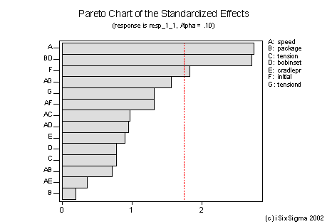
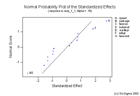
Both the graphs indicate that the main factors of significance are:
- Factor A – speed
- Factor F – initial yarn quality, and
- Interaction B*D (package and bobbin setting)
However let us recollect that this is a Resolution IV design, so confounding exists. We need to study the alias structure carefully before making any conclusions. The alias structure is given below:
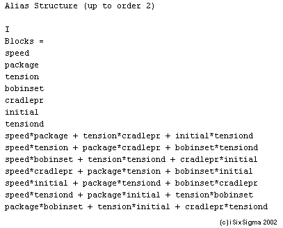
By utilizing the hierarchical ordering principle we can conclude that speed and initial yarn quality are significant factors as they are confounded by three factor interactions.
On viewing the interaction between package and bobbin setting we find that it is aliased as below:
package*bobinset + tension*initial + cradlepr*tensiond
By utilizing the effect heredity principle we see that although [package*bobbin setting] was shown as significant in the pareto diagram, neither package or bobbin setting are themselves significant ruling out the possibility of this interaction being significant. The only interaction in the alias which has at least one factor significant is [tension*initial] wherein initial yarn is significant. Thus the significant interaction is [tension*initial] and not [package*bobbin setting].
The information gathered above is further validated by Interaction graphs and engineering logic.
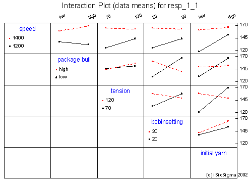
As seen above it was relatively easy to analyze the experiment by use of the three principles. Based on this information we can now fit a reduced model. We can validate our various assumptions by verifying the residuals as below:


In residual analysis there are primarily three points to look at:
- In residual versus time order check for stability over time. The residuals should indicate a random scatter. There should not be any trends in the residuals.
- In the Residuals versus fitted values we check for constancy of variance. This graph should also show a random scatter. If any trends observed, some transformation of data technique will probably need to be applied.
- The residuals should be normally distributed as the third requirement.
It is essential to validate these assumptions before attempting to build the mathematical model.
In our example the residual analysis show no alarms, so we can now look at the mathematical model fitted which is given below:

Based on the mathematical model fitted above we can make predictions about the response:
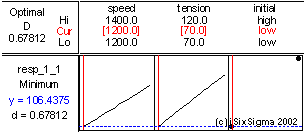
We can now run our confirmation trial and verify whether the predictions made by the model and the actual conditions tally.
Thus if we utilize the three fundamental principles of factorial effects:
It is possible to analyze most Resolution III and IV Design of Experiments without having to run the equal number of earlier run trials but with the signs reversed (also known as a fold over).
Reference
Wu, C. F. Jeff Wu and Michael Hamada, 2000. Experiments: Planning, Analysis, and Parameter Design Optimization. First edition: Wiley-Interscience.