
Censored data is commonly used in reliability studies to determine the mean time to failure in order to establish warranty and maintenance periods for products. A large number of samples are subjected to either normal-use or accelerated-use conditions. Failure modes and occurrences are logged.
Plotting the distribution of the sample failures over time allows the prediction of the mean time to failure for the product being tested. If the warranty period is fairly short, or the manufacturer can wait until all the products fail before establishing the warranty period, then the testing is run until all products fail. If the failures require a long running time, and the product goes to market before all the products fail, then censored data analysis is used to predict the mean time to failure. The data is tagged to indicate whether the data point represents a sample that has failed or whether on the date the data is collected the sample is still operating. If the sample is still operating, the data point is considered to be censored.
Based on the data that has failed, the model establishes the likely failure points for the population of samples – predicting how much longer any censored samples will continue to operate. In Table 1, windings at 80 degrees Celcius failed at an average of 48 months, yet there is one sample still running at 99 months. Based on the remainder of the data (not shown in this table), 15 percent of the windings survive at least 99 months. Looking only at failed data points can skew the understanding of the actual performance of the population.
| Table 1: Example of Censored Data | ||
| Winding at 80 C | Time (Months) | Censor |
| 1 | 50 | 1 |
| 2 | 60 | 1 |
| 3 | 53 | 1 |
| 4 | 40 | 1 |
| 5 | 51 | 1 |
| 6 | 99 | 1 |
| 7 | 35 | 1 |

Transactional processes behave in a similar fashion, if the terminology is translated. Consider booking sales orders. In the process, a salesperson visits a potential customer and attempts to match the customer with a product on offer. In some situations, booking the order is rapid; the customer knows what they want, the salesperson can offer it, the price is accepted and the order is taken. In other situations, there may be negotiations or difficulties in matching the right product with the customer. It may take several contacts between the salesperson and the customer before the order can be booked. All of these sales visits that are pending a received order are censored – the end date is still unknown. If the booking has already become an order, then the event is no longer censored. Sales visits that do not result in an order have failed.
For example, Table 2 shows a number of customer contacts. Six of these contacts have resulted in an order in hand. These orders took an average of 1.3 days to close. There are three customer contacts still pending – no order received. These are censored data points. Sales still expects to receive an order from these customers, although the data in this table suggests that the pending sales contacts may never result in an order. Should the sales team move on to other contacts?
| Table 2: Censored Data Points in Example of Sales Process | ||
| Sales Contact Date | Time Elapsed (Days) | Censor |
| 1/8/2016 | 4.0 | Order received |
| 1/12/2016 | 0.5 | Order received |
| 12/4/2015 | 38.9 | Pending |
| 1/12/2016 | 0.3 | Order received |
| 1/9/2016 | 3.4 | Pending |
| 1/9/2016 | 2.9 | Order received |
| 12/24/2015 | 18.7 | pending |
| 1/9/2016 | 2.9 | Order received |
| 1/12/2016 | 0.1 | Order received |
Companies frequently predict bookings to establish production plans and sales visit schedules. Being able to predict how long to continue to work a potential customer based on the likelihood of achieving a sale can improve the efficiency of the salesforce. Capturing failure modes related to no receipt of an order can help salespeople adjust their approach to potential customers. Understanding the order projection can also help to adjust Sales’ efforts over the course of the reporting period. For example, if the mean time to close an order is two weeks (or two visits) and the end of the reporting period is approaching, it will be better for Sales to focus efforts on bookings that are in progress over efforts to land new customers.
How Censored Data Analysis Works
Censored data analysis requires that a mix of censored and uncensored data be available. In reliability studies, the start time is known for all the samples and at any point in time after that start time, each sample can be assessed as having reached its failure point or as still running. The distribution of all the data points, censored and uncensored, is understood through the science of the product performance, distribution analysis techniques, or using the flexible Weibull distribution.
The bathtub curve represents the typical life of a population of a product (Figure 2). Some products fail early due to flaws in manufacture or assembly. The surviving product samples enter a long period of useful life. Finally, the samples begin to fail and when the failure frequency accelerates, the end of useful life has been achieved. Business decisions determine how to set break-in, maintenance and warranty periods for the product.

Survival plots, cumulative failure plots and hazard plots can all be generated from this analysis to select the accepted level of risk for warranty coverage, preventive maintenance cycles and the like.
Distribution Probability Plot
The distribution probability plot establishes the distribution of the censored and uncensored data, as shown in Figure 3.
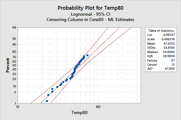
The motor winding data fits the lognormal distribution fairly well – a “fat” pen would cover all the data points. Note that many distributions cannot handle negative or zero value data points.
Survival Plot
The survival plot in Figure 4 shows how many samples are still running over the duration of the testing period.

Cumulative Failure Plot
Conversely, the cumulative failure plot in Figure 5 shows how many samples have failed over the duration of the test.

Hazard Plot
The hazard plot in Figure 6 shows how the rate of failures changes over time. In this case, the rate of failures continues to increase from about 20 months up to 90 months. Between 90 and 120 months, the failure rate is stable. After 120 months, the failure rate begins to decline.

Censored data analysis predicts when failure will occur for the population based on the non-censored and censored results to date. If many censored data points have exceeded the time on the non-censored results, the cumulative failure plot will shift to the right predicting longer life for the samples that have not yet stopped. When we consider only the non-censored data points, the prediction will be a much shorter lifetime, in this scenario.
For transactional processes, such as the sales booking example, the same math works and the same interpretation applies. Today, look at the sales orders and bookings for the month and there are some orders already booked. There are a number of other bookings that have not yet turned into orders. In addition, there is a gap between orders, pending orders and the goal for the month. What needs to happen during the remainder of the month to be certain that the number of orders meet the goal?
The model created from prior analysis of the transformation of bookings to orders can provide confidence in the month’s performance and direct the attentions of sales people to the bookings most likely to become orders. Expanding the model can assure that time is properly spent between this month’s orders and future orders.
Elapsed Time and Censored Data
Survival Plot
A survival plot shows the probability that a sample will survive to a particular age. Depending on the nature of the science behind the life of the sample, the shape of the curve will vary. A survival plot on bookings would show the likelihood that a booking will result in an order at any given point in time. The data shown in Figure 7 that half of sales contacts are still pending an order after nearly 5 days, and 5 percent are still waiting to become an order at 155 days.

Cumulative Failure Plot
In comparison, the cumulative failure plot shows the probability that failure has occurred at a particular point in time. A cumulative failure plot on bookings would show the likelihood that a booking has become an order at any point in time. Figure 8 shows that 50 percent of contacts booked orders in about 5 days and 95 percent booked orders in 155 days. Given that the failure modes for transactional processes are events such as receiving an order or making a delivery, it is common for the cumulative failure plot to be easier and more meaningful to discuss.

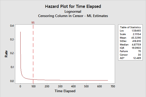
Hazard Plot
Perhaps the hazard plot is the most useful in this case. The hazard to be looking for is when bookings turn into a big waiting game. At what point should a sales contact ever turning into a booked order be given up? At about 95 days, there is a point of diminishing returns. The last 8 percent of unresolved sales contacts trickle in over 608 days, as shown in Figure 9.
Why Include Censored Data Points?
Analyzing with – or without – the censored data points is dependent on a number of factors. First and foremost is the mix of censored and non-censored data points at any given point in time. As the data available on any given day approaches mostly non-censored, then the influence of the censored data is minimal. The mix of factors that we want to analyze, however, must also be proportionately represented in the non-censored data. Other factors to consider include the significance of the differences in the analysis based on the shape of the distribution. If looking at a comparison of statistics associated with the non-censored and total data set for the above sales bookings data, misdirection can occur when ignoring the censored data.
| Table 3: Comparison of Data at Different Time Points | ||
| Order Received (Days) | All Data (Days) | |
| 85 Percent Booked Orders | 23 | 49 |
| 50 Percent Booked Orders | 6 | 5 |
Here is another example to demonstrate the difference between capability including, and excluding, censored data. The bane of many meeting facilitators is getting people to return from break on time. Consider participants receiving a 10-minute break. Track the time when each participant returns and at the end of the break time calculate the average break time for the group. There will be a different break performance than if those who return late from break are included. In Table 4, if looking only at uncensored data, it is possible to believe that the average break time for participants is 8.4 minutes and that the participants are 100 percent compliant. However, after 10 minutes, only 60 percent of the participants are back for the next session. Looking at the full data set, the average break time per participant is 10.1 minutes.
| Table 4: Example of Including, and Excluding, Censored Data | |||
| Participant | Break Duration (Minutes) | Average Break Duration for Group (Minutes) | Percentage Break Less Than or Equal to 10 Minutes |
| 1 | 7 | =7/1=7 | 100% |
| 2 | 8 | =(7+8)/2=7.5 | 100% |
| 3 | 8 | =(7+8+8)/3=7.7 | 100% |
| 4 | 9 | =32/4=8 | 100% |
| 5 | 10 | =42/5=8.4 | 100% |
| 6 | 10 | =52/6=8.6 | 100% |
| 7 | 11 | =63/7=9 | =6/7=86% |
| 8 | 11 | =74/8=9.3 | =6/8=75% |
| 9 | 13 | =87/9=9.7 | =6/9=67% |
| 10 | 14 | =101/10=10.1 | =6/10=60% |
Example – Expense Report Accounting
An accounts payable department experienced a lot of rework to properly allocate expenses to the ledgers when books closed without expense reports in hand. Department managers found their actual expenses did not match their expectations and later changed as accounts payable chased down late expense reports and reallocated expenses to the correct accounts. The baseline data for the project showed 68 percent of expense reports closed within the required 34 days of the charge. Thirty-two percent of the expenses reports had expenses that were subject to reallocation once the reports were finally successfully submitted.
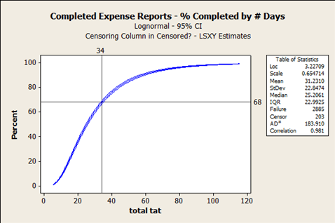
The table of statistics shows that 2,885 of the expense reports achieved “failure,” meaning that they were successfully closed and accounted properly. Another 203 expense reports are tagged as “censor,” which refers to expense reports that have not yet closed. These censored data points are distributed along the entire curve. Some have been open for a day or two while others have been pending for weeks.
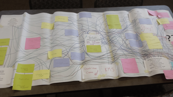
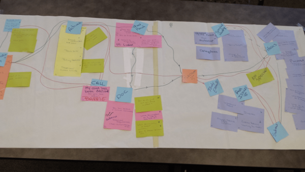
When the expense report team investigated the various stages of the reporting process (purchase, create and submit the report, report approval, and final accounting audit) the stage with the longest cycle time was creating and submitting the report. An investigation into the demographics of the report creators (departments, positions/roles, types of expenses, etc.) showed that there were no particular culprits. Many individuals were rare submitters. An investigation into the follow-up on expense reports that had to be revised showed that the real root cause of the long submittal time was that the rules for allocating the charges and completing the expense report correctly were confusing for the purchasers – experienced and inexperienced alike. A spaghetti diagram showed that getting questions answered was a long, convoluted process.
This process was simplified by putting all of the information in the same place, accessible to all. Individuals with questions, or individuals who submitted faulty expense reports, were directed to that source.
The final results of this action in Figure 13 show the improvement in expense report cycle times.
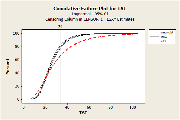
When the cumulative failure curve shifts to the left, the speed of the operation is faster. In this case, the number in compliance with the 34-day target climbed to 81 percent, which was deemed “good enough.” Perhaps the best outcome was when a key individual in accounting complained that the managers were taking too long to approve the reports and another project was needed; the manager approval cycle time was less than 2 days, including weekends.
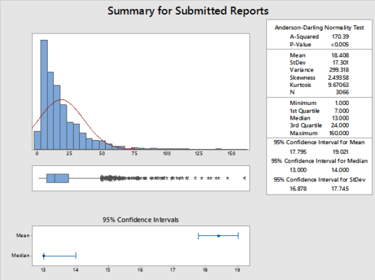
If the censored data points had not been considered, the accounts payable department would never have worked to solve the problem. A comparative group of only closed reports shows a mean of 18 days and 85 percent of the submitted reports complying with the 34-day specification. Including the censored data points in the analysis properly weights the tail of the distribution. In this case there was a bias associated with early failures (that is, successfully submitted reports) that pulled the data that excludes censored data into shorter times, as shown in Figure 14.
Conclusion
Trusting the data is fundamental to process excellence, but it is also important to ensure that the data is being analyzed in contexts that reveal all it has to share. While analyzing failure rates generally provides useful information, in transactional processes where long cycle times are possible, looking only at failed data points can skew the understanding of the actual performance of the population. Censored data analysis can help provide a more accurate understanding.