
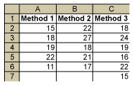
Three methods used to dissolve a powder in water are compared by the time (in minutes) it takes until the powder is fully dissolved. The results are summarized in the following table:
It is thought that the population means of the three methods m1, m2 and m3 are not all equal (i.e., at least one m is different from the others). How can this be tested?
One way is to use multiple two-sample t-tests and compare Method 1 with Method 2, Method 1 with Method 3 and Method 2 with Method 3 (comparing all the pairs). But if each test is 0.05, the probability of making a Type 1 error when running three tests would increase.
A better method is ANOVA (analysis of variance), which is a statistical technique for determining the existence of differences among several population means. The technique requires the analysis of different forms of variances – hence the name. But note: ANOVA is not used to show that variances are different (that is a different test); it is used to show that means are different.
How ANOVA Works
Basically, ANOVA compares two types of variances: the variance within each sample and the variance between different samples. The following figure displays the data per method and helps to show how ANOVA works. The black dotted arrows show the per-sample variation of the individual data points around the sample mean (the variance within). The red arrows show the variation of the sample means around the grand mean (the variance between).

The assumption is: If the population means are different, then the variance within the samples must be small compared to the variance between the samples. Hence, if the variance between divided by the variance within is large, then the means are different.
Steps for Using ANOVA
Step 1: Compute the Variance Between
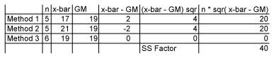
First, the sum of squares (SS) between is computed:
![]()
Where x-bar is the sample mean and x-double-bar is the overall mean or grand mean. This can be easily found using spreadsheet software:
Now, the variance between or mean square between (ANOVA terminology for variance) can be computed.
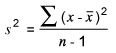
The formula for sample variance is:
Since there are three sample means and a grand mean, however, this is modified to:
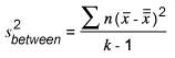
Where k is the number of distinct samples. In other words, the variance between is the SS between divided by k – 1:
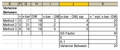
(This example uses Microsoft Excel software. In Minitab software, SS between is called SS factor, variance between is called MS factor and K – 1 is called DF.)
Step 2: Compute the Variance Within
Again, first compute the sum of squares within. This is:
![]()
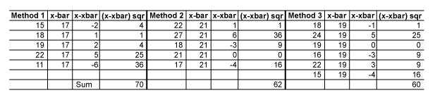
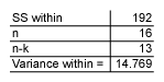
SS within is 70 + 62 + 60 = 192.
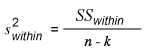
To obtain the variance within, use this equation:
Step 3: Compute the Ratio of Variance Between and Variance Within
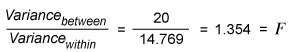
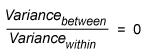
This is called the F-ratio. How can this be interpreted? If the null hypothesis is true, meaning m1, m2 and m3 are all equal, then the variance between the samples is 0 (zero) (i.e., the F-ratio is also zero).
If the null hypothesis is not true, then this F-ratio will become larger, and the larger it gets, the more likely it is that the null hypothesis will be rejected.
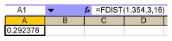
Using the F-tables for k = 3 and n = 16, one gets a p-value of 0.292 (use the FDIST function in Excel). This means that the probability that the observed F-ratio of 1.354 is random is 29.2 percent:
Hence, if one sets a = 0.05, one must accept the null hypothesis that there is no difference in the population means.
In Minitab, the results for the same data are displayed in the session window like this:
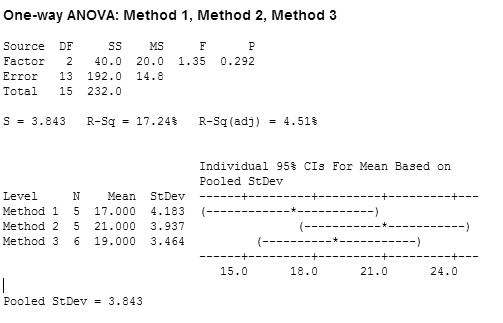
If there had been a significant difference between the samples, this would have been seen with the p-value and also there would have been at least one confidence interval for one mean that had no, or very little, overlap with the other confidence intervals. This would have indicated a significant difference between its population mean and the other population means.
Minitab also computes an R-squared value (R-Sq) by taking the SS factor/SS total = 40/232 *100 = 17.24. This shows the percent of explained variation by the factor. Here, the factor only explains 17.24 percent of the total variation; hence, it is not a very good explanation.