Over the past 25 years, design of experiments (DOE) has enjoyed increasing application in manufacturing and service industries in the improvement of products, processes and service quality. The method is used to conduct experimental runs for identifying the best settings in multiparameter problems. Although experimentation can be a costly process, great potential is usually uncovered wherever engineering teams use DOE to drive improvement. Therefore, it is important that new Belts get a good grasp of this concept.
One tool for teaching this method is simulated designed experiments. Through simulations, new Belts can get hands-on experience while learning the challenges of DOE, before they apply it to costly real-world experiments.
Classic Teaching Methods
Lean Six Sigma trainings typically introduce DOE as follows:
- Simple examples for fundamental understanding
- Case studies
- Practical exercises using a wooden catapult or paper helicopters to show the concepts of mathematical modeling.
After trainings using this method, engineers sometimes remain reluctant to shoulder the responsibility of conducting designed experiments in their own working environment. Because of the direct experience gained through simulated DOEs, using this method may help in overcoming that barrier.
Design of a Function for a Simulated DOE
Data for simulated designed experiments is produced by a model known by the instructor but unknown to students. This model should:
- Be easy to understand so the instructor can design it quickly.
- Be sufficiently complex such that students cannot guess it.
- Allow for the inclusion of interaction and non-linear effects and noise.
Such a model can be built with a function of three variables: X1, X2 and X3. The directions for completing the model are:
1. Set f(X1, X2, X3) = aX12 + bX22 + cX32 + f0 with a global maximum (or minimum) if a, b and c are smaller (or greater) than zero. In cases where at least one coefficient has a sign different from the others, f(X1, X2, X3) has no extreme. It can be rewritten as f(X) = XTAX + f0,
where X = (X1, X2, X3) and A has a, b and c as diagonal elements, while non-diagonal elements vanish. Then A = AT (AT is the transposed matrix of A).
2. Shift f(X) by setting X’ = X-X0 to create linear terms.
3. Apply a sequence of rotations to create interaction-terms: y = PX’,
where P can be a rotation matrix using Euler angles, which represent the spatial orientation of a frame. The function then reads:
f(y) = yTPTAPy – 2X0TPTAPy + X0TPTAPX0 + f0
It displays linear and non-linear terms. Original function and rotation can be programmed into a spreadsheet program, where noise also can be added.
Simulation Example
The following description presents a DOE example an instructor employed during a training class. The area of interest to be explored is between the corner points (±1, ±1, ±1).The function is set as f(X1, X2, X3) = X12 + 2X22 + 3X32 + 10, with a global minimum of 10 at (X1, X2, X3) = (0,0,0). It is shifted to have its new minimum at (X1, X2, X3) = (0.2, 0.3, 0.4) and rotated around the z- and x-axis, and again around the z-axis by 30° each. This provides a new function:
f(X1, X2, X3) = 10.45 – 0.45X1 – 0.24X2 – 1.84X3 – 1.08X1*X2 + 0.17X1*X3 – 1.15X2*X3 + 1.78X1*X1 + 1.53X2*X2 +2.69X3*X3.
Between the corner points, the highest value is found to be 16.9 and the lowest 10.1 (resulting in a range of about 6.8). Now, 20 percent of that range is added as noise to the function’s values.
Experiment
The team decides to run a full-factorial design with one replicate per corner point and four center points, for which the instructor provides the function’s values.
Had the center points not been included into the first run, it would have been impossible to detect curvature. The result would have been indistinguishable from a situation where the optimum is outside the area of interest.
Now that curvature is present, the response optimizer within a typical statistical analysis software program shows the optimum is close to the center of the cube. The team decides to run a block of axial points together with two more center points.
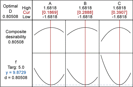
Output from the response-optimizer for the complete data set from 20 experimental runs is shown in the figure below. The minimum is found at (X1, X2, X3) = (0.19, 0.29, 0.39), close to the “real” minimum at (0.2, 0.3, 0.4).

Reviewing the Model
Now it is possible to compare the best-fit function with the original model. Within the area of interest, the mismatch between the two is below 2 percent. This also is reflected in the match of the model parameters (see table below).
| Model Coefficients as Set by the Instructor (Original) and as Determined by the Team (Best Fit) | ||||||||||
| F0 | X1 | X2 | X3 | X12 | X22 | X32 | X1*X2 | X1*X3 | X2*X3 | |
| Original | 10.45 | -0.45 | -0.24 | -1.84 | 1.78 | 1.53 | 2.69 | -1.08 | -0.17 | 1.15 |
| Best Fit | 10.30 | -0.42 | -0.28 | -1.72 | 1.83 | 1.55 | 2.73 | -1.07 | 0 | -1.17 |
Many Simulation Uses
Simulated designed experiments offer a welcome variation in DOE trainings. Besides the application described here, teams can use simulations to:
- Compare different DOE designs (Box-Behnken, Face-centered, Taguchi and so on).
- Set extremes outside the area of interest (leading to evolutionary operation, where static operation of a process is replaced by a continuous and systematic slight changes in the control variables).
- Study the power of DOE designs in the presence of different levels of noise.
The key advantage of simulated designed experiments is the fact that data from known models can be analyzed and the result can be compared to it so that possible traps are understood before a DOE is set up in a costly real-world experimental context.