Optimize Attribute Responses Using Design of Experiments

The objective of a design of experiments (DOE) is to optimize the value of a response variable by changing the values, referred to as levels, of the factors that affect the response. Although often a response is continuous in nature, there are some cases in which the response falls in the attribute category (e.g., pass/fail, accept/reject, etc.). This article explains how to analyze an attribute type of response, using an example from the manufacturing sector.

Example Experiment

In this example there are three factors with two levels. The factors are renamed as Factor1, Factor2 and Factor3, and the levels are coded as -1, +1.

The experiment was conducted with 10 replicates, or repetitions of the experiment at each combination of level settings, to provide greater accuracy for attribute data.

In this example, the total number of runs was L^F x replicates = 23 x 10 = 80, where L = number of levels and F = number of factors.

A single set of experiments with 10 replicates is shown in Table 1.

Table 1: Results of 10 Replicates with 1 Combination of Levels
Factor1	Factor2	Factor3	Response
-1	+1	-1	OK
-1	+1	-1	NOK
-1	+1	-1	OK
-1	+1	-1	OK
-1	+1	-1	OK
-1	+1	-1	OK
-1	+1	-1	OK
-1	+1	-1	OK
-1	+1	-1	OK
-1	+1	-1	OK

Next, the responses for the replicates of this experiment were converted into proportions, p. In the results shown in Table 1, the proportion of OK (okay) to NOK (not okay) was 9 out of 10. Thus, p = 0.90.

Once the experiment was conducted for all combinations of levels, the captured OK/NOK attribute responses were converted into proportions, displayed in Table 2.

Table 2: Summary of Experiment Data for All Combinations of Levels
Factor1	Factor2	Factor3	p
-1	-1	1	0.70
1	-1	-1	0.00
-1	1	-1	0.90
1	1	1	0.60
1	1	-1	0.40
-1	1	1	1.00
1	-1	1	0.00
-1	-1	-1	0.10

Arcsine Function

The arcsine square-root transform is the variance stabilizing transform for the binomial distribution and is the most commonly used transformation. It assists when working with proportions and percentages. The proportion, p, can be made nearly normal if the square root of p is used with the arcsine (or inverse sine: sin^-1) transform. The arcsine transform is then computed as a function of p ? arcsin (sqrt(p)).

In the example, the calculated p was converted into sqrt(p) and then again converted into arcsin (sqrt(p)) by using the arcsine function. The results are shown in Table 3.

Table 3: Updated Results with Arcsine Function
Factor1	Factor2	Factor3	p	Sqrt(p)	*Arcsin (sqrt(p))*
-1	-1	1	0.70	0.83666	0.99116
1	-1	-1	0.00	0.00000	0.00000
-1	1	-1	0.90	0.94868	1.24905
1	1	1	0.60	0.77460	0.88608
1	1	-1	0.40	0.63246	0.68472
-1	1	1	1.00	1.00000	1.57080
1	-1	1	0.00	0.00000	0.00000
-1	-1	-1	0.10	0.31623	0.32175

Analysis of Results

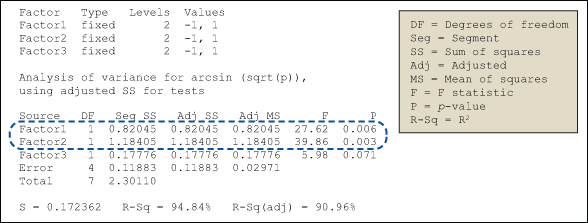
The general linear model (GLM) in analysis of variance (ANOVA) was used to identify the significant factor(s) among the three factors. The arcsine value was specified as the response, and Factor1, Factor2, Factor3 were provided as the factors. The output of GLM is shown in Figure 1.

Figure 1: General Linear Model: Arcsin (Sqrt(p)) Versus Factor1, Factor2, Factor3

The p-value calculated within the GLM results indicates that Factor1 and Factor2 are statistically significant. That is, those factors have a significant bearing on the arcsine value.

Interaction Plot

An interaction plot displays the mean of the response variable for each level of a factor with the level of a second factor held constant. Interaction plots are useful for judging the presence of interactions – when the response at one factor level depends upon the level(s) of other factors.

Parallel lines in an interaction plot indicate no interaction; non-parallel lines indicate an interaction between the factors. The greater the departure of the lines from the parallel state, the higher the degree of interaction. To produce an interaction plot, data must be available from all combinations of levels.

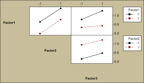
An interaction plot for the sample data is shown in Figure 2.

Figure 2: Interaction Plot for Arcsin (sqrt(p))

In all cases in Figure 2, the interaction lines are parallel, which shows there are no significant interactions between the factors.

Main Effects Plot

A main effects plot is used in conjunction with ANOVA and DOE to examine differences in the response variable at varying levels for one or more factors. When different levels of a factor affect the response differently, a main effect is present. A main effects plot graphs the response mean for each factor level connected by a line.

The general patterns to look for are:

When the line is horizontal (parallel to the x-axis), there is no main effect present. Each level of the factor affects the response in the same way, and the response mean is the same across all factor levels.
When the line is not horizontal, then there is a main effect present. Different levels of the factor affect the response differently. The steeper the slope of the line, the greater the magnitude of the main effect.

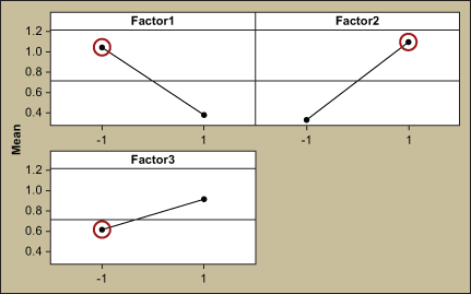
The sample data is shown in a main effects plot in Figure 3 and suggests that a main effect is present in Factor1 and Factor2 as the lines are not horizontal.

In the example, a larger value of the response arcsin (sqrt(p)) represents a better outcome. With that in mind, the analysis suggests that the levels -1 for Factor1, +1 for Factor2 and +1 for Factor3 will provide the desired results (i.e., high proportion of acceptance, or low proportion of rejections).

Figure 3: Main Effects Plot for Arcsin (sqrt(p))

Response Optimization

Response optimization is a method of analysis to identify the combination of input variable settings that jointly optimize a single response or a set of responses. Within a statistical analysis program, the response optimizer function provides an optimal solution for the input variable combinations, and sometimes an optimization plot. The optimization plot may be interactive, in which case the input variable settings can be adjusted on the plot to search for more desirable solutions.

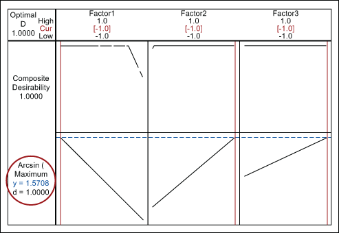
Figure 4 shows the results of the response optimizer analysis for the example data. It indicates that the maximum arcsine is 1.5708 with a desirability of 1.

Solution and Verification

Based on the results of the analysis, the process parameters for factors are set at the following levels to reduce the number of rejections:

Factor 1: -1
Factor 2: +1
Factor 3: +1

To verify the above settings, 30 experiments were conducted and resulted in 0 rejections. With that verification, the process settings were approved and updated in all appropriate process documents.