When analyzing data as part of a Lean Six Sigma project, some Belts can become confused to the point of fear when their coach tells them they need to perform a hypothesis test. This fear often comes from two sources: 1) the selection of the appropriate hypothesis test and 2) the interpretation of the results.
But using hypothesis tests does not need to be scary. By breaking down the process and keeping several reminder charts on hand, Belts can ease their fear of using these powerful statistical tools.
Determining Normality
Not all data is normal. But many Lean Six Sigma students are told to assume normality because it makes the job of analyzing data easier. This is far from the truth, especially when practitioners focus on projects calling for process cycle-time reduction, which involve data that is typically not normal. With hypothesis testing, Belts must know whether or not the data is normal as different tests apply in different circumstances.
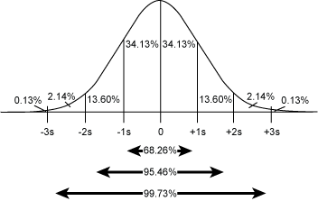
So the first step is to determine normality. Normal data is defined as data that has “normal” variation. This means that it will take the shape of a standard bell curve. The bell curve represents the central tendency of the data. The distribution also will follow these rules (as shown in Figure 1):
- Plus or minus 1 standard deviation around the mean contains roughly 68 percent of all data
- Plus or minus 2 standard deviation around the mean contains roughly 95 percent of all data
- Plus or minus 3 standard deviation around the mean contains roughly 99.7 percent of all data

It is these properties that enable a practitioner to use a tool called a probability plot to determine if data is normally distributed. A probability plot is a graphical, or visual, method to show normality, but, unlike the histogram, it is based on a statistical test.
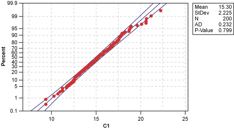
Specifically, the probability plot is a graph on semi-log paper (i.e., the y-axis is not linear) which plots the value on the x-axis and the percent of the data that any specific value is relative to the distribution. For example, in Figure 2, the mean on the x-axis of around 15 will translate to 50 percent on the y-axis; in other words, 50 percent of the data is below the mean and 50 percent is above the mean.

To interpret this chart, if the data is distributed throughout the range of the measurement following a random variation pattern, a practitioner would expect 50 percent of the data to fall to the lower side of the median, 50 percent above the median and so on. The breakdown would follow the percentages listed in the picture of the normal curve in Figure 1. In a probability plot, this would result in a straight line, plotting the value of the data on the x-axis and the percentage less than the value of the data point on the y-axis.
Normal data would therefore approximate a straight line, as shown in Figure 2, indicating that as the value increases, a higher percentage of the total data falls within that range.
As a rule of thumb, if 80 to 90 percent of the data points fall between the lines, a practitioner can conclude that the data is normal.
The probability plot serves as the first key point for determining which hypothesis test to use.
Selecting the Appropriate Test
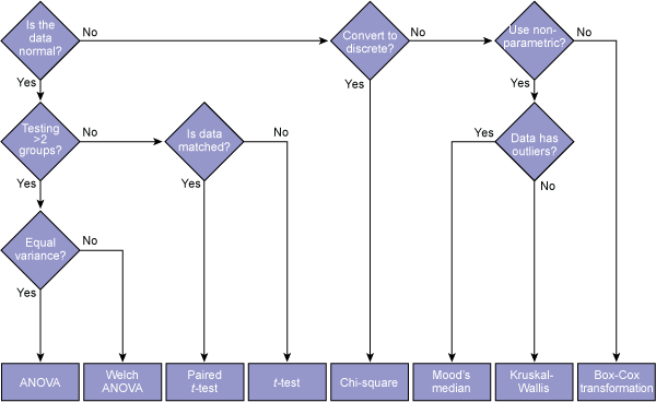
At this point in the analysis, Belts need to decide on a direction to follow and the type of hypothesis test to use. For the inexperienced Belt, this can be an overwhelming task. Using the flow chart in Figure 3 can help determine the appropriate test to use.

The following example can assist Belts in using the flow chart:
A Belt is analyzing why three different manufacturing lines that produce the same product have different cycle times. The data pulled showed that all lines have a normal variation, but with different means. The Belt is attempting to determine if this difference is statistically significant or just part of normal variation. In this case, statistically significant means the difference is not due to common-cause variation.
Following the flow chart, the data is normal for each line as determined from probability plots, so the Belt moves to the next decision: Is this a comparison of more than two groups? The answer is yes because the Belt is looking at three lines. Again, the Belt continues down to the next decision: Do the groups have equal variances? Here, the Belt needs to perform an F-test or a test for equal variances. If the results of the test determine that the groups have equal variances, the Belt proceeds down the chart and uses ANOVA.
It is important to note that if the data is not normal, there are different avenues that can be taken. For example, using the same example above of comparing cycle times of three manufacturing lines, assume the data was not normal. Moving to the right on the flow chart, the next question is: Can you convert the data to discrete? In other words, can the Belt convert the individual continuous data points to discrete data by comparing them to a specification or by “bucketing” the data into groups? Doing that will result in a contingency table, which could be used in a chi-square test. The chi-square test would help determine which line is not performing like the others using discrete data instead of continuous data.
If converting to discrete data is not an option, there is a group of tests known as non-parametric hypothesis tests, such as Mood’s median test or the Kruskal-Wallis test, which deliver the same results for non-normal data. In almost all cases, these are a good alternative.
Lastly, if, for some reason, conversion to discrete data is not possible and the Belt cannot use non-parametric tests, they can convert the data using a Box-Cox transformation.
Interpreting the Results
Most Green Belts and Black Belts hear the statement, “Just look for the p-value” when being taught how to interpret the results of a hypothesis test. The p-value is what practitioners look to in order to determine if they should reject or fail to reject the null hypothesis (H0). The H0 almost always involves the statement, ”There is no difference between groups.”
To clarify this, Belts can use the chart below.
Table 1: How to Interpret Test Results
| Test Name | Purpose of Test | p-value < 0.05 | p-value > 0.05 |
| Two-sample t– and paired t-test | Test if the difference between two means is statistically significant | Reject H0, confirming a difference exists | Fail to reject H0, confirming no difference exisits |
| One-way ANOVA, Welch ANOVA | Test if the difference between two or more means is statistically significant | Reject H0, confirming at least one mean is different | Fail to reject H0, confirming no difference exists |
| Kruskal-Wallis | Test if the difference between two or more medians is statistically significant, if data has outliers | Reject H0, confirming a difference exists | Fail to reject H0, confirming no difference exists |
| Mood’s median | Test if the difference between two or more medians is statistically significant | Reject H0, confirming a difference exists | Fail to reject H0, confirming no difference exists |
| Chi-square | Test if the difference between two or more group proportions is statistically different | Reject H0, confirming at least one group is different | Fail to reject H0, confirming no difference exists |
| F-test (Bartlett’s for normal data, Levene’s for non-normal data | Test if the difference between two variances is statistically different | Reject H0, confirming a difference exists | Fail to reject H0, confirming no difference exists |
Note that if the hypothesis test confirms that a difference exists, all that has been proven is that a difference exists. It is now up to the Belt to look at the details of the process and use investigative skills to identify the potential causes for the difference.