Process capability (Cp) studies are usually performed whenever:
- Engineering tolerances are reviewed against the observed variability of the process and/or new equipment is evaluated,
- The capability of a process to meet customer specifications needs to be determined or
- Process changes and/or improvements need to be evaluated.
Our rapid pace and highly competitive industrial environments often require expeditious decisions/actions in the above areas and an automated statistical method which minimizes sampling during these studies would be highly desirable. The sequential test method for process capability decisions described below will often result in a 50 percent sampling saving when compared with the most powerful classical tests. It is also both computer user and spreadsheet software friendly.
Applying Wald’s Sequential Test Method to Process Capability Decisions
A process is defined as capable when the determined statistical control limits are at least equal to or within the specification limits and deemed incapable whenever the control limits lie outside of the specification limits. The capability index
![]() where the upper specification limit (USL) and lower specification limit (LSL) represent the upper and lower specification limits and s the population standard deviation (STD), is a handy measure of process capability.
where the upper specification limit (USL) and lower specification limit (LSL) represent the upper and lower specification limits and s the population standard deviation (STD), is a handy measure of process capability.
By convention, if Cp < 1, the process is deemed incapable; if Cp = 1 or Cp > 1, the process is considered marginally or definitively capable (e.g., Cp >= 1.33). Hence, for a selected USL-LSL specification range, any sampling decision on whether a process is capable is dependent upon the process standard deviations s0 (Cp > 1 ) s1 (Cp < 1 ) and corresponding Type I a and Type II b errors for hypothesis acceptance or rejection. With the exception of double sampling, most accept/reject inspection decisions assume that the observational numbers are independent of the results and require a predetermined sample size. Sequential test or inspection plan sample sizes are dependent on the outcome of the observations and require three decisions: 1) accept the test hypothesis, 2) take another observation and 3) reject the test hypothesis.
Historically, sequential testing results from the theory of sequential analysis that was created by WALD2 in 1943 for war time military equipment development and inspections. Numerous examples of the theory’s practical applications and sampling saving economies were later published1 by the Statistical Research Group of Columbia University. Examples of the mentioned 50 percent sampling economy can be found in the document. The basis for Wald’s sequential test are the probability inequality ratios:
 where P0N, P1N are the probability density functions corresponding to the test H0 and alternate H1 hypothesis for the sequential set of observations X1…XN, and a, b are the selected Type I (producer’s risk) and Type II (consumer’s risk) errors. The test is continued when inequality ratio (2) applies and discontinued at the first occurrence of the ratios (1) or (3) resulting in the acceptance of hypotheses H0 or H1 respectively.
As an example of test principle usage, consider the sequence of observations X1…XN from a normally distributed process with a known mean m and unknown standard deviation s, where the test hypothesis is s = s1. For each value of N, the probability ratio P1N/PON is calculated. Thus, the test hypothesis s = s1 when (3) P1N/PON >= (1-b)/a. The test is continued when (2) b/(1-a) < P1N/PON < (1-b)/a. The expansion of inequality (2) results in expression (4) below:
 and further simplification results in the straight line forms that are used to create the table (Table 2) and/or graph (Figure 1) of a Wald sequential test procedure for process variability:
Accept standard deviation s0 at step N if the summed observations * S (Xi – m)2 satisfy
![]()
and continue sampling if
![]()
where:
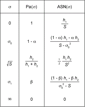
 *Note: In the cases where the mean m is unknown the sum of squares is replaced by the squares of the deviations from the sample mean and the limit N is replaced by N-1. Five useful points of both the operating characteristic Pa(s) and ASN curves can be calculated from the formulas in Table 1.

The ASN estimates the average number of samples required for a decision at a specified standard deviation s since the exact number is not known beforehand.
A Process Capability Application Example1
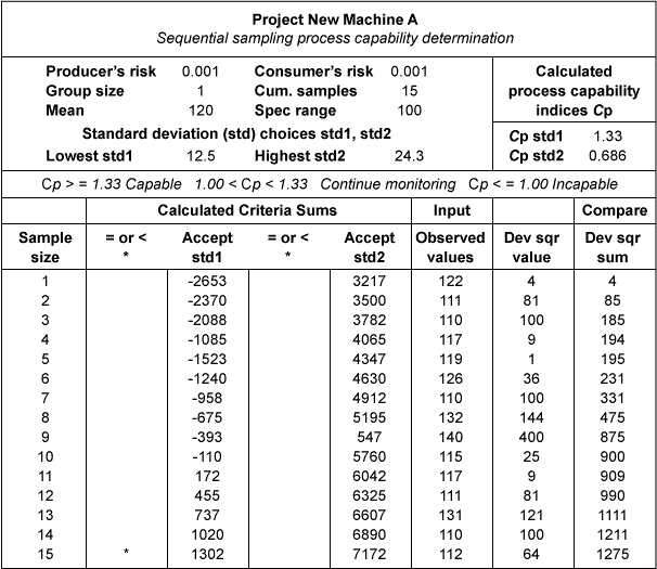
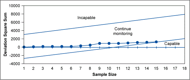
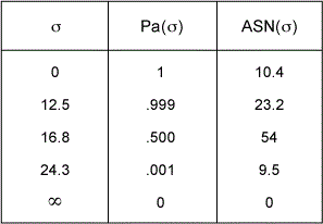
A textile customer specifies an average burst strength and tolerance of 120 pounds +/- 50 pounds for each patch of manufactured cloth and further requires a minimum Cp of 1.33. The specification range (USL-LSL) in this case is 100 pounds and the maximum allowable process standard deviation calculates as 100/(6 x 1.33) = 12.5 pounds. The cloth manufacturer accepts the customer’s specification based on a standard deviation comparison of New Machine A with the historical results obtained for older equipment. The sequential sampling parameters s0=12.5, s1=24.3, a=0.001 and b=0.001 are chosen for the study. The Excel spreadsheet outputs are illustrated in Table 2, Figure 1 and Table 3. Table 3 lists an ASN of 23 for this test at the desired standard deviation level of 12.5. The test was terminated after 15 cumulative samples were taken. This is indicated by the asterisk in the immediate left column of the calculated accept STD1 (12.5) criteria sums in Table 2 and Figure 1 chart. The manufacturer has decided to produce the customer’s orders on New Machine A (Cp >= 1.33) since the older equipment is not capable.


Variance Sampling Economy
When a classical test of significance is applied to question of whether the sample variance s2 differs significantly from the desired population variance s0, a Chi-square test X2 is usually applied. The test hypothesis H0 specifies the population variance as H0: s2 = s02 and the alternate hypothesis H1: s12 > s02. If H0 is correct, then X2/f is the distribution for s2/s02 for f degrees of freedom. Thus, a rejection of the test hypothesis H0 occurs at some chosen significance level a such that
Method Limitations Versus Advantages
A limitation4 of the sequential method is that compensations are not made for the effects of sample grouping on Type I, Type II errors, ASN and OC curve values. When compared with single item sequential plans, grouping by sample increments results in an increase in the number of items inspected and advantageously lower Type I and Type II errors. If the process is evaluated is very good or bad, expeditious decisions occur. However, these accept or reject decisions are dependent upon the closeness of the standard deviation parameters s0, s1 and the degree of risk a, b that the manufacturer or organization is willing to accept. Borderline processes often require indefinite sample sizes and a truncation point leading to an increased a or b risk has to be agreed upon. The method does not exempt the manufacturer or organization from continuous monitoring since processes do change in time. Also, the example discussed is based on the assumption of a centered normally distributed process.
Aside from sampling economy, the major advantage in the use of Wald’s sequential probability ratio test (SPRT)5 arises from the ease at which it can be automated, enhanced and extended to the binomial, Poisson and reliability test areas. Algorithms can be devised that require only computer familiarity and data entry skills on the part of the user. Additionally, hardware as simple as a programmable pocket calculator can be used for many of the applications.
References
1. Statistical Research Group, Columbia University (1945). “Sequential Analysis of Statistical Data: Applications,” Columbia University Press, New York, NY. The exhibit data from section 6.216 was used to validate output from Excel Spreadsheet formulas. The standard deviation and type I, II error input parameters were varied for example purposes.
2. Wald, A (1947), Sequential Analysis, John Wiley & Sons, New York, NY.
3. Hald, A (1952), Statistical Theory with Engineering Applications, John Wiley & Sons, New York, NY.
4. D. R. Garrison, J. J. Hickey, Journal of Quality Technology, Vol 16, No. 3 July 1984, “Wald Sequential Sampling for Attribute Inspection.”
5. Additional SPRT citations can be found at http://citeseer.nj.nec.com/context/78315/0 and Internet Interactive Wald Sequential Sampling Tables for Attributes can be generated at http://home.clara.net/sisa/sprthlp.htm.