In manufacturing, key quality indices – performance capability index (Cpk), defects per million opportunities (DPMO) and first pass yield (FPY) – are prevalent criteria for gauging the performance of products and processes. These indices however, often are interpreted wrongly and used without taking into account the conditions of application. Moreover, alternative indices such as rolled throughput yield (RTY) are sometimes ignored. The following case studies illustrate the proper use of Cpk, DPMO and FPY, and can be used as a guide for practitioners who apply these indices.
Problems with Cpk
Despite the importance placed on Cpk, continuous improvement practitioners often face problems when applying this indicator.
Losing Sight of Distribution
Cpk is calculated based on the premise that a process is controlled statistically (stable) and that product data follows normal distribution. Processes can be deemed in or out of control based on process data compiled in an Xbar-R chart. The process is out of control if:
- A single point exceeds the 3 sigma control limits.
- At least seven successive points fall on the same side of the centerline.
- Seven successive points occur in ascending or descending order.
Cpk is typically calculated using this equation:
![]() , where
, where
Estimated process standard deviation ![]() ,
, ![]() is the process mean,
is the process mean, ![]() is the mean range value, d2 is a constant decided by subgroup size, and LSL and USL stand for lower specification limit and upper specification limit, respectively.
is the mean range value, d2 is a constant decided by subgroup size, and LSL and USL stand for lower specification limit and upper specification limit, respectively.
The following case study illustrates the application of Cpk in conjunction with an Xbar-R chart. Supplier A produces rubber pads with a thickness specification between 7.56 mm and 8.32 mm. In order to evaluate the performance of the process, 45 finished products are randomly chosen for analysis (Figure 1).

The Xbar-R chart produced in the analysis demonstrates that the process is under control. Nonetheless, the normal probability plot, which specifically tests normal distribution, shows that the 45 samples apparently do not conform to normal distribution because the p-value (0.005) is far less than 0.05. Based on hypothesis testing, if the p-value is less than 0.05, then the practitioner can reject the null hypothesis that the population follows normal distribution. The capability histogram also displays the pattern of non-normal distribution. Therefore, the Cpk value 0.53 virtually fails to mirror the truth of the process performance, proving the Cpk statistic should be ignored when data distribution is substantially not normal.
In real-world situations, it’s common for raw data not to be distributed normally; usually it fits other distribution patterns such as lognormal, exponential or Weibull. Statistical analysis software was used to verify whether the 45 samples from this case followed Weibull distribution (Figure 2).

The data did not conform to Weibull distribution with a 95 percent confidence interval, and the p-value (0.018) is far less than 0.05. Upon further analysis, the data is proven not to conform to either lognormal or exponential distribution. Under these circumstances, Box-Cox transformation is used to transform the data before Cpk is calculated (Figure 3).

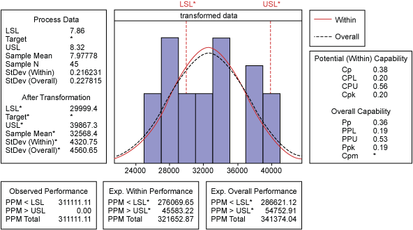
Ultimately, Cpk turned out to be 0.20, which is dramatically different from the value 0.53 before transformation. However, the curves in Figure 3 disclosed that the transformed data remained non-normally distributed. That is, the raw data was characterized by irregularity, so there was no point in computing Cpk. In this case, non-conforming DPMO was used to gauge process performance. Figure 3 shows the short-term DPMO and long-term DPMO was approximately 322,000 and 341,000 respectively.
Based on this case study, it is unreasonable to calculate Cpk directly without considering the distribution pattern. Furthermore, an Xbar-R chart is an indispensable tool for monitoring process status and should be required for analysis. As for supplier A, its rubber pads are made from scrap tires. Most of the time, scrap tires have been abraded unevenly and some chunks of tire may have come off; therefore, uniform thickness is not guaranteed, which is why the small Cpk emerged. From a manufacturing perspective, one approach to enhance the Cpk value of the process would be to fabricate rubber pads out of raw rubber instead of scrap tires. Of course, the additional cost from this process change should be taken into consideration. Because of the narrow profit margin for rubber pads, it is inadvisable to control the Cpk value of the process beyond 1.33, as long as thickness is qualified.
Multiple Machines and Operators
In mass production, various operators using multiple identical machines aim to make identical products, which all must meet set thresholds in characteristics such as shaft diameter and sheet thickness. Accordingly, disparities in operators’ skills and machine performance are worth consideration when calculating Cpk.
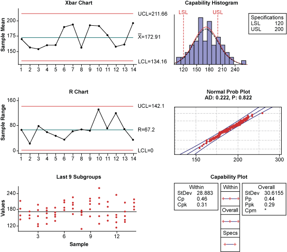
The following case study illustrates this importance: In a compressor factory, two operators are assigned to spray paint on crankcases manually. Each operator possesses a spray gun. All of the wet paint is prepared by a process engineer. A quality inspector routinely completes random checks of 10 crankcase surfaces for paint thickness. In order to determine the spraying process capability, seven units painted by two operators also are randomly chosen to spot check the paint thickness (Figure 4).

The normal probability plot in Figure 4 shows a p-value of 0.822, which is greater than 0.05, signifying that thickness measurements on Oct. 24 follow normal distribution. However, the histogram signals bimodal distribution – the mixture of two normal distributions. The root cause for such a phenomenon is the use of two spray guns. Bimodal distribution is commonplace in processes where two pieces of manufacturing equipment are employed. Care should be exercised when multiple identical machines are allocated to produce the same parts because distribution may appear non-normal. As a result, it is difficult to troubleshoot if data is not categorized by machines and operators.
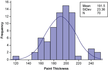
In this case, one operator was well trained and experienced, while the other had comparatively less experience. Also, one of the operators was usually in a hurry to complete the spraying task, so the irregular distribution of paint thickness is not surprising (Figure 5). Thus, the Cpk value calculated under these conditions is misleading.

For quality control, it is much better to carry out Cpk analysis classified by operator in order to distinguish the abilities of different operators. To diagnose capability of equipment, the measurement Cmk (machine capability index) should be used:
![]() , where
, where
s is standard deviation of samples and  .
.
The difference between Cpk and Cmk lies in the denominator of the equations. Commonly, machine capability is acceptable when Cmk is greater than 1.67. In the case of paint thickness, if the Cmk of the two spay guns greatly differ from each other, the thickness data of crankcases painted by these two spray guns would conform to bimodal distribution. Note that Cmk calculation is based on the assumption that variability in materials, human factors and environment have been removed.
Problems with DPMO
DPMO is the most frequently used yardstick for evaluating product quality. In terms of quality management, DPMO is often associated with defect percentage of a certain population. One example of its application: In a factory where chillers are produced, the DPMO equation is
DPMO = (defective units/total units sold) x 1,000,000
In general, the total units sold monthly ranges from 200 to 700. Table 1 shows the relation between total units sold and defective units at various sigma quality levels. Note that a shift of 1.5 sigma is considered when converting sigma into DPMO.
| Table 1: Relation Between Total Units Sold and Defective Units | |||||
| Sigma Level | Total Units Sold Monthly | Defective Units | Sigma Level | Defective Units | Total Units Sold Monthly |
| 4 sigma | 161 | 1 | 3 sigma | 210 | 14 |
| 4 sigma | 322 | 2 | 3 sigma | 449 | 30 |
| 4 sigma | 805 | 5 | 3 sigma | 704 | 47 |
| 4.5 sigma | 7,411 | 1 | 3.5 sigma | 220 | 5 |
| 4.5 sigma | 1,482 | 2 | 3.5 sigma | 703 | 16 |
This table indicates that the factory cannot reach a 4.5 sigma quality level unless at least 741 units are sold monthly with only one nonconforming unit, or at least 1,482 units are sold monthly with no more than two defective units. Because a rate of zero defects is rare, the paramount driver for achieving 4.5 sigma level is total units sold. In other words, a combination of market demand and sales volume is the decisive factor in raising sigma quality level. Of course, there is a chance that 4 sigma level in this factory can be met if proper actions from engineering, manufacturing and management are taken and the process is monitored strictly.
Practitioners should calculate DPMO based on the category of components, such as compressors, valves and so on. For the factory here, each chiller is equipped with four compressors, the component with the highest defect rate. Suppose 700 units of chillers (2,800 compressors) are sold monthly and 10 compressors have quality problems. The DPMO of nonconforming compressors amounts to 14,286. This metric is more meaningful as opposed to the total DPMO of nonconforming chillers because it assists in prioritizing projects for quality improvement. Undoubtedly, factories always put more energy into addressing issues that take up the largest portion of quality cost. Calculating the DPMO of an individual issue helps decision makers gain an insight into each issue and solve problems in a cost-efficient way.
Problems with FPY
The metric FPY is used to assess the performance of a process; rework and repairs are not a part of FPY calculation. Once rework is in the picture, rolled-throughput yield (RTY) is a better metric. RTY is obtained by multiplying together the qualification rates of each process step.
For instance, suppose 100 units go through 10 operations in an entire process (Figure 6). Throughout the process steps, faulty units are detected. Some can be repaired and returned to the operation, while others are scrapped.

In this case, FPY = 96/100 = 96 percent, because four units are scrapped throughout the whole process. However, RTY = (100-4)/100 x (99-3)/99 x (97-3)/97 = 90.2 percent of units passed the first inspection. Six percent of the units will be reusable after repair. RTY is more informative than FPY, because RTY conveys the qualification rate of each workstation as well as the general picture of scrap, rework and repair. Practitioners should calculate both FPY and RTY for a panoramic view of overall process quality.
Know the Metrics
The quality indices Cpk, DPMO and FPY should be used extensively in numerous enterprises; however, the computation of metrics should not turn into a superficially mechanical task. Rather, practitioners should take time to understand fully the application conditions. They must also keep in mind the value of Xbar-R charts and alternative performance metrics, such as RTY.