
© Oakland Images/Shutterstock.com
Key Points
- The Plackett-Burman design method is one of the most useful tools when you don’t have all the data available for an experiment.
- They cannot show any correlation between data sets without a clearer picture.
- They are useful for screening or seeing where certain factors might influence the outcome of a process.
Plackett-Burman experimental design is used to identify the most important factors early in the experimentation phase when complete knowledge about the system is usually unavailable.
Developed in 1946 by statisticians Robin L. Plackett and J.P. Burman, it is an efficient screening method to identify the active factors using as few experimental runs as possible.
In Plackett-Burman designs, the main effects have a complicated confounding relationship with two-factor interactions. As such, these designs should be used to study the main effects when it can be assumed that two-way interactions are negligible.
In practical use, two-level full or fractional factorial designs, and Plackett-Burman designs are often used to screen for the important factors that influence process output measures or product quality.
However, these designs are useful for fitting first-order models (which detect linear effects). Accordingly, they can provide information on the existence of second-order effects (curvature) when the design includes center points.
Full Factorial Experiment
To demonstrate the effectiveness of the Plackett-Burman design, an experiment was conducted to compare a full factorial experiment with a Plackett-Burman design. Let’s start with the full factorial experiment, which consists of five factors with two levels for each factor.
With this in mind, the total number of experiments is 25 = 32 (Table 1). The characteristic of the response, Y, is the larger the better.
| Table 1: Five Factor Analyses with Two Levels (Full Factorial Design) | |||||
|
A |
B |
C |
D |
E |
Y |
|
-1 |
-1 |
-1 |
-1 |
-1 |
75.87 |
|
1 |
-1 |
-1 |
-1 |
-1 |
76.14 |
|
-1 |
1 |
-1 |
-1 |
-1 |
109.95 |
|
1 |
1 |
-1 |
-1 |
-1 |
109.55 |
|
-1 |
-1 |
1 |
-1 |
-1 |
80.17 |
|
1 |
-1 |
1 |
-1 |
-1 |
80.3 |
|
-1 |
1 |
1 |
-1 |
-1 |
114.07 |
|
1 |
1 |
1 |
-1 |
-1 |
114.05 |
|
-1 |
-1 |
-1 |
1 |
-1 |
68.77 |
|
1 |
-1 |
-1 |
1 |
-1 |
68.63 |
|
-1 |
1 |
-1 |
1 |
-1 |
102.41 |
|
1 |
1 |
-1 |
1 |
-1 |
102.27 |
|
-1 |
-1 |
1 |
1 |
-1 |
72.95 |
|
1 |
-1 |
1 |
1 |
-1 |
72.68 |
|
-1 |
1 |
1 |
1 |
-1 |
106.98 |
|
1 |
1 |
1 |
1 |
-1 |
106.65 |
|
-1 |
-1 |
-1 |
-1 |
1 |
75.79 |
|
1 |
-1 |
-1 |
-1 |
1 |
75.71 |
|
-1 |
1 |
-1 |
-1 |
1 |
110.08 |
|
1 |
1 |
-1 |
-1 |
1 |
110.04 |
|
-1 |
-1 |
1 |
-1 |
1 |
80.49 |
|
1 |
-1 |
1 |
-1 |
1 |
80.86 |
|
-1 |
1 |
1 |
-1 |
1 |
113.49 |
|
1 |
1 |
1 |
-1 |
1 |
114.06 |
|
-1 |
-1 |
-1 |
1 |
1 |
68.22 |
|
1 |
-1 |
-1 |
1 |
1 |
68.6 |
|
-1 |
1 |
-1 |
1 |
1 |
102.5 |
|
1 |
1 |
-1 |
1 |
1 |
102.3 |
|
-1 |
-1 |
1 |
1 |
1 |
73.03 |
|
1 |
-1 |
1 |
1 |
1 |
73.3 |
|
-1 |
1 |
1 |
1 |
1 |
106.08 |
|
1 |
1 |
1 |
1 |
1 |
106.7 |
Normal Plot
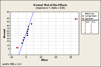
The primary goal of screening designs is to identify the vital few factors or key variables that influence the response. A normal plot is one of the graphs that help identify these influential factors.
Accordingly, in the normal probability plot of the effects, points that do not fall near the line have measured values that are significantly beyond the observed variation, and usually signal important effects. Important effects are larger and generally further from the fitted line than unimportant effects. Unimportant effects tend to be smaller and centered around zero.
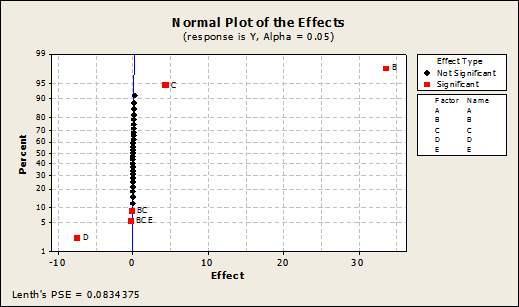
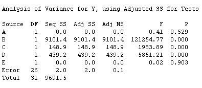
As shown in the normal plot (Figure 2) and the analysis of variance (ANOVA, Figure 3), the factors B, C, and D are significant to the response. Additionally, there are two-way interactions between factors B and C and three-way interactions among B, C, and E.
Main Effects Plot
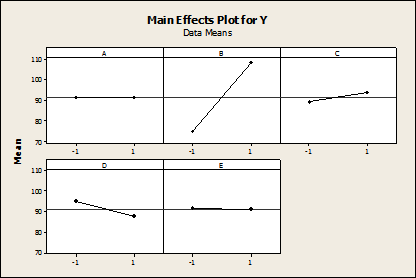
In experimental design, a main effects plot is used in conjunction with ANOVA to examine differences among level means for one or more factors. It graphs the response mean for each factor level connected by a line. As can be seen, a main effect is present when different levels of a factor affect the response differently (shown as a slope on a two-level plot).
Some general patterns to look for with main effects plots include the following:
- When the line is horizontal (parallel to the x-axis), then there is no main effect present. Each level of the factor affects the response in the same way, and the response mean is the same across all factor levels.
- When the line is not horizontal, then a significant main effect may be present. Different levels of the factor affect the response differently. The greater the slope, the greater the likelihood that a main effect is statistically significant.
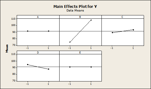
The factors B, C, and D are shown to be significant to the response Y as shown in Figure 3.
Response Optimization
The Response Optimizer function in Minitab helps to identify the combination of input variable settings that jointly optimize a single response or a set of responses. (Note: Minitab requires the user create a starting point for the optimization and will find the first best solution based on the requested optimization objective.) This function provides an optimal solution for the input variable combinations and an optimization plot. The optimization plot is interactive – input variable settings on the plot can be adjusted to search for more desirable solutions.
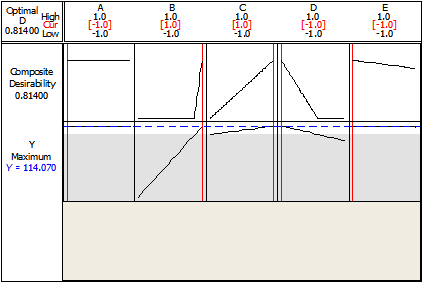
The nature of the response, Y, is “the larger the better” – and the maximum value that can be achieved in this experiment is 114.07, as shown in Figure 4.
That means to achieve the maximum value of Y, the process variables should be set as shown in Table 2.
| Table 2: Levels of Process Variables (Full Factorial Design) | ||
|
Variable |
Optimal Level |
Notes |
|
A |
-1 | A is insignificant and might not create high impact if it is changed to +1 |
|
B |
+1 | |
|
C |
+1 | |
|
D |
-1 | |
|
E |
-1 | E is insignificant and might not create high impact if it is changed to +1 |
Plackett-Burman Experiment
Having completed the two-level full factorial experiment, let’s turn to the Plackett-Burman experiment for comparison. In this experiment, five factors with two levels are considered. The total number of experiments is selected to be the minimum from the Plackett-Burman design – 12 experiments (Table 3). Remember that for Y, the larger the better.
| Table 3: Five Factor Analysis with Two Levels (Plackett-Burman Design) | |||||
|
A |
B |
C |
D |
E |
Y |
|
1 |
-1 |
1 |
-1 |
-1 |
75.67 |
|
1 |
1 |
-1 |
1 |
-1 |
102.4 |
|
-1 |
1 |
1 |
-1 |
1 |
113.71 |
|
1 |
-1 |
1 |
1 |
-1 |
72.95 |
|
1 |
1 |
-1 |
1 |
1 |
102.32 |
|
1 |
1 |
1 |
-1 |
1 |
113.85 |
|
-1 |
1 |
1 |
1 |
-1 |
106.51 |
|
-1 |
-1 |
1 |
1 |
1 |
72.66 |
|
-1 |
-1 |
-1 |
1 |
1 |
68.62 |
|
1 |
-1 |
-1 |
-1 |
1 |
75.54 |
|
-1 |
1 |
-1 |
-1 |
-1 |
109.28 |
|
-1 |
-1 |
-1 |
-1 |
-1 |
75.69 |
Breaking Down the Plackett-Burman Design
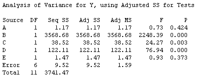
As shown in the normal plot in Figure 5, factors B and D are significant. As shown in Figure 6 with ANOVA, factors B, C, and D are significant to the response Y. It is important to note that the significance of interactions is not displayed as Plackett-Burman’s design is interested only in the main effects.
The main effects plot (Figure 7) shows that the factors B, C, and D are significant to the response Y.
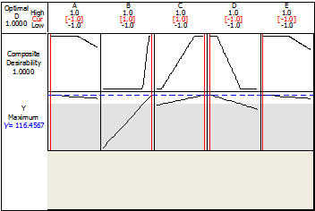
The nature of the response, Y, is the larger the better, and the maximum value that can be achieved in this experiment, according to the Response Optimizer (Figure 8), is 116.46.
Thus, to achieve the maximum value of Y, the process variables should be set as shown in Table 4.
| Table 4: Levels of Process Variables (Plackett-Burman Design) | ||
|
Variable |
Optimal Level |
Notes |
|
A |
-1 | E is insignificant and might not create a high impact if it is changed to +1 |
|
B |
+1 | |
|
C |
+1 | |
|
D |
-1 | |
|
E |
-1 | E is insignificant and might not create high impact if it is changed to +1 |
Why It Matters
Hypothesis testing is a crucial part of any project. However, you might not have all the data available for an expected result right off the bat. As such, the Plackett-Burman allows you to readily run a test to see if there are significant influences that might sway the outcome of a given process.
Comparison of the DOE Results
A comparison of the results obtained from both the full factorial design of experiments and the Plackett-Burnam design of experiments is shown in Table 5.
| Table 5: Comparison of Results | ||
|
Full Factorial Design |
Plackett-Burman Design | |
| Number of experiments |
32 |
12 |
| Significant factors |
B, C, D |
B, C, D |
| Significant levels |
B: +1, C: +1, D: -1 |
B: +1, C: +1, D: -1 |
| Significant interactions |
(B, C) and (B, C, E) |
Non-detectable |
| Optimized value of Y |
114.07 |
116.46 |
There is no difference in significant factors or significant levels, but there is a slight difference in the optimized value of Y. The factor settings and conclusion remain the same when using either design, but there is a significant difference in the number of experiments that need to be conducted to achieve these results.
When to Use Plackett-Burman Design
It is particularly helpful to use the Plackett-Burman design:
- In screening
- When neglecting higher-order interactions is possible
- In two-level multi-factor experiments
- When there are more than four factors (if there are between two to four variables, a full factorial can be performed)
- To economically detect large main effects
- For N = 12, 20, 24, 28 and 36 (where N = the number of experiments)
Drawbacks of Plackett-Burman Design
There are also some drawbacks to using Plackett-Burman designs that practitioners should be aware of:
- They do not verify if the effect of one factor depends on another factor.
- If you run the smallest design you can, it does not follow that enough data has been collected to know what those effects are precisely.
Other Useful Tools and Concepts
There are plenty of useful tools at the ready when going through your DOE process. I heavily recommend looking into the details behind the full factorial design. While we touch on it briefly here, it isn’t an exhaustive or comprehensive look at the subject.
Additionally, you might want to see how DOE impacts any given process. Kienle + Spiess has utilized Lean Six Sigma DOE to transform the quality of its welds. You can see how they’ve done it in our informative post-mortem taking a look at the steps they took.
Conclusion
Plackett-Burman design is helpful if complete knowledge about the system is unavailable or in the case of screening with a higher number of factors. However, once the significant factors are available and the interactions between the factors are required, it is better to go with full factorial design as it takes the combinations of all the levels between the factors and provides the interaction details.