Can we trust the data? This is the fundamental question behind measurement system analysis (MSA). The question can come up in any data-based project. Shortcomings in a measurement system’s accuracy (bias, linearity, stability or correlation) and precision (resolution, repeatability or reproducibility) can obstruct analysis purposes.

One often-overlooked aspect of resolution is data granularity, or the measurement increment. Compared to other aspects of MSA, granularity is straight-forward to identify and relatively easy to fix. However, ignoring the importance of granularity may unnecessarily limit root cause analysis and the ability to manage and continually improve a process.

Granularity Makes a Difference

Simulated data from an imaginary delivery process is used here to illustrate the role of granularity. An exponential distribution is assumed for two suppliers, A and B, where the scale of the distribution is 70 and 90 hours, respectively. For supplier A, 20 percent of its deliveries (one day out of five) see a normally distributed additional delay of 100 hours, with a standard deviation of 20 hours. This could be due to delay accumulated in deliveries initiated the last day of the week.

To understand the impact of granularity, 250 data points from each of suppliers A and B are rounded up to hourly and daily resolution. Practitioners then complete the analysis by:

1. Visualizing the data
2. Identifying the data’s underlying distributions
3. Testing the suppliers’ influence on spread and central tendency

Visualizing the Data

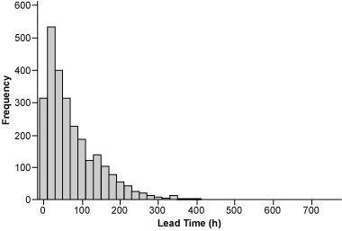
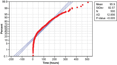
Probability plots are far more capable than histograms of revealing data granularity. For this purpose, normal probability plots also can be used for non-normal data, as in this example. The histograms (Figure 1) and probability plots (Figure 2) of the cumulated data from both suppliers A and B with hourly resolution (above) and daily resolution (below) are shown here. Notice that the additional delay in 20 percent of the data is barely visible in the histogram of the hourly resolution data and not visible in the data with daily resolution.

Identifying Individual Distributions

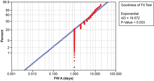
Because it is known how the data has been produced, the question is whether the differences between suppliers A and B can be revealed. A powerful method to start the data analysis is to identify the underlying distributions. In this situation, the method yields results only for the data with hourly resolution (Figure 3): unlike the data from supplier B, the data from supplier A does not fit to any distribution. Daily resolution does not offer insight into the shape of the distribution (Figure 4).

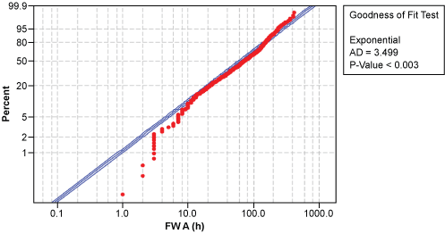
Thus, viewing data with appropriate granularity (in this example, hourly resolution appears to be sufficient) allows practitioners to find differences between the two data sets. Improvement teams can then conduct further investigation by asking “why?” and identifying special causes for the differences, such as the additional delay of shipments from supplier A one day a week.

When dealing with data with inappropriate granularity (in this example, daily resolution is of too low a granularity), neither set of data can be described by any distribution and special causes remain invisible (Table 1).

Table 1: Summary Results of Individual Distribution Identification
	Supplier A	Supplier B
Hourly resolution	No best-fit distribution with P > 1 percent	Gamma, Exponential and Weibull distributions fit with P-values > 25 percent
Daily resolution	No best-fit distribution with P > 1 percent	No best-fit distribution with P > 1 percent

Testing Spread and Central Tendency

Studying spread and central tendency are other methods used to reveal differences. However, they are less powerful than the individual distribution identification; multiple distributions, as well as mixed or merged distributions like the data for supplier A, can have the same spread or central tendency. Thus, individual distribution identification has a stronger discrimination power.

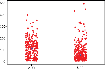
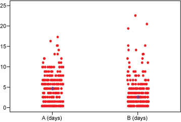
For non-normal data, the appropriate tests for spread and central tendency are Levene’s and Kruskal-Wallis (or Mood’s median), respectively (Table 2). The central tendency test uses the median if data is non-normal, as in the current situation (Figure 5).

Table 2: Results of Statistical Tests for the Two Sets of Data
	Hourly Resolution	Daily Resolution
Spread (Levene’s test)	A: 80.7 hours B: 82.4 hours (P-value = 4 percent)	A: 3.36 days B: 3.43 days (P-value = 4 percent)
Central Tendency (Kruskal-Wallis test)	A: 108.5 hours B: 57.5 hours (P-Value = less than 1 percent)	A: 5 days B: 3 days (P-Value = less than 1 percent)

Differences in spread were found to be marginally significant (P-value = 4 percent) from a statistical point of view. But both sets of data led to the conclusion that supplier B is faster. However, without the knowledge gained through the individual distribution identification, it is impossible to attribute this either to common cause variation (variation due to the nature of the distribution, such as Gamma, Weibull or exponential) or to special cause variation (like the “Friday effect” in the current example).

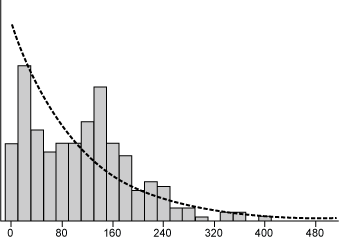
Another way to look at differences is to stratify the data by suppliers A and B within histograms. The special cause known to be active for supplier A becomes visible only in the data with hourly resolution (Figure 6), where two modes – which originate from the mixed nature of the underlying lead time distribution – are visible. Important indications may thus be overlooked if the data is of too low a granularity.

Finding the Right Granularity

Metrics used for tracking adherence to customer specifications and other process performance standards usually follow ratios of precision to tolerance (P/T). In the context of granularity, the equivalent to precision is the measurement increment.

Practitioners should use the ratio of the measurement increment to the process sigma (spread) as a way to quantify the impact of granularity on the ability to detect special causes of variation. As a rough guideline, this ratio should be smaller than 10 percent for granularity to be acceptable, where a ratio much smaller than 10 percent is preferable. A ratio greater than 30 percent would be unacceptable.

For the tolerance window, defined by the customer specification limits, similar requirements hold: in order to tell whether a value is within or outside the specification limits, the measurement increment must be smaller than a tenth of the width of the tolerance window. Notice that, in conjunction with the first requirement, this only has practical relevance in cases of poor process capability when the tolerance window is about as wide as or even wider than the process spread.

Table 3 summarizes these parameters for the two data sets with hourly and daily granularity where the tolerance is given by an upper specification limit of 5 days (120 hours). For lead time data, the lower bound is zero. Clearly, the measurement system with a daily increment is at best marginally acceptable both from a customer’s perspective and from a process perspective.

Table 3: Acceptability of Granularity
	Tolerance (T)	Spread	Measurement Increment (MI)	MI/T	MI/Spread
Hourly resolution	120 hours	83 hours	1 hour	0.8 percent	1.2 percent
Daily resolution	5 days	3.4 days	1 day	20 percent	29 percent

Taking Action

These observations lead to the following implications:

1. When releasing Measure phase tollgates, namely of lead time reduction projects, Master Black Belts should require a MSA and make sure granularity is considered.
2. A few slides about granularity should be included in the training materials for all Green Belt and Black Belts.
3. Organizations should screen their databases for delivery lead time data. Many companies only store “shipment day” and “reception day” data. This produces lead time data of daily granularity, which can keep practitioners from detecting delays and special causes.
4. In most such situations, providing a sound operational definition of “start” and “end” of the process, along with mapping out the process, can yield immediate improvement potential. This is especially true at beginning and end of a delivery process, where delays may come from letters waiting in signature folders or parcels left in shipment areas.