
Some practitioners mistakenly believe that it is not necessary to transform data before creating an individuals control chart when the underlying process distribution response is not normal. An individuals control chart, however, is not robust to non-normally distributed data. Therefore, it is important to use an alternate control charting approach.
Necessary Transformation
Consider a hypothetical application of the individuals control chart involving an accounts receivable department sending invoices to customers for payment. The difference between payment date and due date often follows a lognormal distribution.
The following data can be considered a random selection of one invoice daily for 1,000 days, where the payment date for the invoice was subtracted from its due date. Therefore, for instance, a positive value of 10 indicates that an invoice payment was 10 days late.
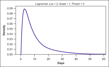
In this example, 1,000 points were randomly generated from a lognormal distribution with a location parameter of 2, a scale parameter of 1 and a threshold of 0 (i.e., lognormal 2, 1, 0). The distribution from which these samples were drawn is shown in Figure 1. In this simplified illustration, it is considered that nobody paid early, where the threshold would be equal to zero. A normal probability plot of the 1,000 sample data points is shown in Figure 2.
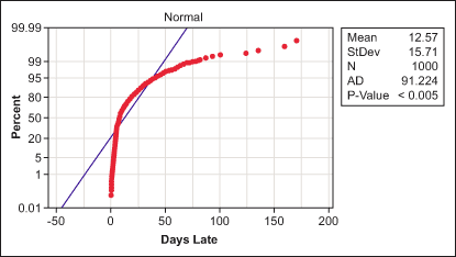
From Figure 2, it is possible to reject the null hypothesis of normality technically, because of the low p-value, and physically, because the normal probability plotted data does not follow a straight line. This is also logically consistent with the problem setting, where a normal distribution for the output of such a process is not necessarily expected. A lognormal probability plot of the data is shown in Figure 3.
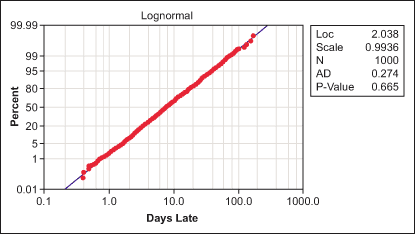
From Figure 3, a practitioner would not reject the null hypothesis of the data being from a lognormal distribution because the p-value is not below the criteria of 0.05 and the lognormal probability plotted data tends to follow a straight line. Hence, it is reasonable to model the distribution of this variable as lognormal.
If the individuals control chart is robust to the non-normality of data, an individuals control chart of the randomly generated data should be in statistical control. In the most basic sense, using the simplest run rule (a point is “out of control” when it is beyond the control limits) such data would be expected to give a false alarm three or four times out of 1,000 points, on average. Further, a practitioner could expect false alarms below the lower control limit to be equally likely to occur as false alarms above the upper control limit.
Figure 4 shows an individuals control chart of the randomly generated data.
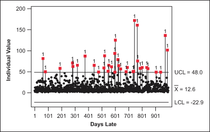
The individuals control chart shows many out-of-control points beyond the upper control limit. In addition, the individuals control chart shows a physical lower boundary of 0 for the data, which is well within the lower control limit of -22.9. If no transformation is needed when plotting non-normal data in a control chart, then a practitioner would expect to see a random scatter pattern within the control limits, which is not the case in Figure 4.
Figure 5 shows a control chart using a Box-Cox transformation with a lambda value of 0, the appropriate transformation for lognormally distributed data.
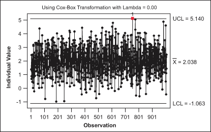
This control chart is much better behaved than the control chart in Figure 4. Almost all 1,000 points are in statistical control. The number of false alarms is consistent with the design and definition of the individuals control chart control limits.
Finding the Process Capability Metric
By using a lognormal probability plot, it is possible to determine the best estimate process capability metric output for this fictitious process: 80 percent of all invoices are paid between 2.1 and 27.4 days beyond the due date, with a median of 7.7 days late, when no specification exists (Figure 6).

If data is not from a normal distribution, an individuals control chart can generate many false signals, leading to unnecessary tampering with the process. When no specifications exist, a best estimate for the 80 percent frequency of occurrence rate, along with median response, is an easy-to-understand description that conveys what the process is expected to produce in terms that everyone can visualize. If a specification exists, then the percentage non-conformance can be determined from the probability plot and be presented as the process capability of the process.
Avoiding Type 1 Errors
The specific distribution used in the prior example, lognormal (2, 1, 0), has an average run length (ARL) of 28 points for type 1 errors (when the null hypothesis is rejected in error). The single sample used showed 33 out-of-control points, close to the estimated value of 28. Considering a less-skewed lognormal distribution, lognormal (4, 0.25, 0), the ARL for false rule one errors drops to 101. Note that a normal distribution will have a type 1 error ARL of around 250.
The lognormal (4, 0.25, 0) distribution passes a normality test more than half the time with samples of 50 points. In one simulation, a majority (75 percent) of the type 1 errors occurred on the samples that tested as non-normal. This result reinforces the conclusion that normality or a near-normal distribution is required for a reasonable use of an individuals chart or a significantly higher type 1 error rate will occur.