Six Sigma is the new rallying cry for quality improvement in the process industry. For example, Dow aims to generate an extra $1.5 billion per year in profits after training 50,000 of their employees on the methods of Six Sigma.3 Statistical tools play a key role in achieving savings of this magnitude. In fact, sigma is a Greek letter that statisticians use as a symbol for standard deviation – a measure of variability. If a manufacturer achieves a Six Sigma buffer from its nearest specification, they will experience only 3.4 off-grades per million lots. This translates to better than 99.99966 percent of product being in specification. To illustrate what this level of performance entails, imagine playing 100 rounds of golf a year with two putts per hole being the norm (par): At Six Sigma you’d make a three-putt (bogey) only every 163 years! Even Tiger Woods would be envious of this level of quality.

Of all the statistical tools employed within Six Sigma, design of experiments (DOE) offers the most power for making breakthroughs. Via an inspirational case study, this article demonstrates how DOE can be applied to development of a formulation and its manufacture to achieve optimal performance with minimum variability, thus meeting the objectives of Six Sigma programs. Armed with knowledge gained from this article and the example as a template, chemists and engineers from any of the process industries (pharmaceutical, food, chemical, etc.) can apply these same methods to their systems and accomplish similar breakthrough improvements.

Minimizing Propagation of Error (POE) from Varying Inputs

After earning his PhD in chemistry and taking a job at a chemical company, a colleague of ours got assigned to an operator for an orientation to the real-world of production. As the operator watched with much amusement and disgust, the chemist carefully weighed out materials with a small scoop. The operator pushed the PhD chemist aside, grabbed a sack of chemicals and tossed it into the reactor. “You’re not in the laboratory anymore,” he said, “This is how we do things in manufacturing.”

Hopefully the operators of your formulation process will be more exacting when adding ingredients. However, at the very least, you can expect some variation due to inherent limitations in equipment. How will these variations affect product quality and process efficiency? Can you do anything to make your system more robust to variations in component levels and process settings? The answers to these very important questions can be supplied via an advanced form of DOE called response surface methods (RSM). This statistical tool produces maps of product and product performance, similar to topographical displays of elevation, as a function of the input variables that you (or your clients) control. The objective of Six Sigma is to find the flats – the high plateaus of product quality and process efficiency that do not get affected much by variations in component levels or factor settings. You can find these desirable operating regions visually, by looking over the 3D renderings of response surfaces, or more precisely via a mathematical procedure called POE.

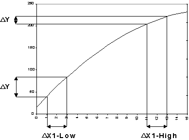
To see how POE works, let’s look at a very simple response surface (Figure 1) generated by changing only one control factor X1.

Assume that this factor exhibits a constant variation shown on the graph as a difference with magnitude delta (D). This variation, or error, will be transmitted to the measured response to differing degrees depending on the shape of the curve at any particular setting. In this example, because the curve flattens out as the control factor increases, a setting at the higher level causes less propagation of error (POE). Therefore, you see a narrower difference (DY) on the response axis as a result of setting the factor at the higher, rather than lower level.

With the aid of some calculus, the POE itself can be graphed as a continuous function. In this case the original response surface can be described by the following quadratic equation:

We will spare you the details, but after taking the partial derivative of this function with respect to the input (X1) and taking the square root, the following equation for standard deviation(s) is produced:

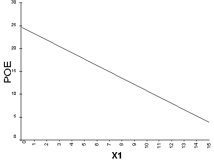
Assume for now that the standard deviation of the control factor X1 equals one (sx = 1) and there are no other sources of variance (sResidual = 0). We’ve now obtained the information needed for graphing the standard deviation of the response transmitted from the variation in the input factor (X), in other words, the POE (see Figure 2). In this case the POE decreases in direct proportion to X1 as it increases.

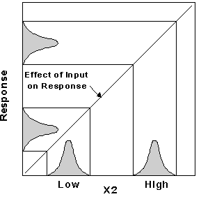
Obviously, reducing response variation is a highly desirable outcome. But, what if the absolute level of response gets shifted out of specification? Ideally you will find another control factor that affects response in alinearfashion, such as that shown in Figure 3. (We added the bell-shaped curves to indicate that variation will likely be distributed according to a normal distribution.)

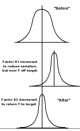
This factor (X2) creates no effect on POE (it is constant), so it can be used to get your response back into specification after changing the other factor (X1) to reduce variability. In this case X2 must be decreased to counteract the increase in response caused by increasing X1 (done to reduce POE). Ideally, as in this simplified example, you can achieve the best of both worlds as shown in Figure 4: on-target response with minimal variability, hopefully to the level demanded by Six Sigma.

Let’s see how these concepts can be applied to a Six Sigma project on a coatings system. We chose this example because anyone can identify with problems of paint peeling (who hasn’t had this happen at home?). However, we expect chemists and engineers in other process industries (pharmaceutical, food, chemical, etc.) to use this as a template for improving their particular formulation and manufacturing procedures.

Part 2 > A Case Study on POE