The goal in product design or business process engineering is to create products or processes that are insensitive to the sources of variation that inhibit their intended function. The design phase in the product development process is a crucial activity since this is when most downstream production and quality problems are locked-in. As a consequence, a successful DMAIC (Define, Measure, Analyze, Improve, Control) Six Sigma program may evolve into what is known as Design for Six Sigma (DFSS).

DFSS integrates marketing, engineering and production information into the design world. DFSS focuses on preventing defects by optimizing a transformation of customer needs into what can be produced in engineering and the process domain. Therefore, DFSS starts by defining a problem in the customer domain to understand the voice of the customer (VOC) and the customer’s use of the products or transactions. Models must then be developed in the engineering or process domain with the help of functional parameter diagram and quality function deployment (QFD)-like techniques. The model must be a translation of the voice of the customer into a system that can be engineered. Understanding design variable interactions and sensitivity of system performances relative to system variables is the ultimate goal of this step.

Having understood the behavior of the system, the next steps are to find optimal and robust solutions and then verify the solutions in customer and production conditions. Typically, DFSS deals with multiple objectives in the optimization step and then stack-up tolerance analysis and degradation or key life testing in the verification step. Robustness and optimal solutions will ensure the product meets the customer’s intended use and is delivered on time and at a lower cost – eventually improving the company’s profitability.

Complexity and Pace Demand Use of Computer Analysis

Complexity of the product or process and the fast-paced schedule to bring the product to market demands that DFSS takes advantage of computer-based analysis. Computer-based analysis needs analytical (either mathematical or simulation) models called transfer function and analytical optimization. Transfer function can be derived from the first principle of physics, engineering drawing of stack-up processes, finite element method-based simulation such as computer aided engineering (CAE), regression analysis of empirical or observational data, and/or response surface from computer experimental designs. When the analytical models do not include comprehensive noise factors such as piece-to-piece variation, changes in dimension or strength over time/cycle, customer usage and duty cycle, external operating environment, and internal operating environment /interaction with neighbouring subsystems, they can be represented by the variability of the existing variables or parameters in the models.

The goal of computer-based experimentation is multiple. One goal is to develop simple approximation that is fast to compute and accurate enough within a certain design space, especially for time-consuming CAE models. Computer-based experiment logistics are often straightforward so that relatively large number of runs may be feasible and parameters can be adjusted in software. A large number of runs allows variable sampling over many levels instead of just fewer runs with limited variable sampling, e.g., two or three in hardware experimentation. Multi-level sampling can capture high order and nonlinear models. Since responses from computer are deterministic, there is no random error, and replication and randomization do not have value. Therefore, flexible alternatives to standard arrays, e.g., uniform design and Latin hypercube designs are suitable to running computer-based experimentation.

Illustrated here is a step-by-step process for executing analytical or computer-based DFSS. This includes identifying voice of the customer, translating VOC to critical-to-quality characteristics (CTQ) using QFD, modeling system transfer function using engineering drawing, finding optimal and robust solutions using graphical approach and mathematical programming based on computer experimentation, and finally indicating tolerance design approach. The case study shows how to find optimal and robust designs of a sliding door. The study can be run using available commercial software. This example can be easily adapted to different product design and business process engineering, including transactional products and processes. The essential difference between engineering and transactional processes is that natural laws, such as conservation of energy or mass, govern engineering and manufacturing processes, but man-made laws, such as regulations, govern transactional processes.

Step 1. Identifying VOC

The first step is identifying the customers’ needs. In the case of the sliding door, customers’ desires have been found to be:

• Good value
• Reliable and durable design for various materials and conditions
• Low noise and rattle level
• Ergonomic features, easy to use with minimum effort to open
• Safety features to prevent accidents

Step 2. Translating VOC to CTQ

QFD in the form of house of quality translates VOC to CTQ. The house of quality below shows that noise and rattle level is related to the clearance between track and roller of the door. When the clearance is too big, the rattle level will increase, but when it is too tight, the noise level will increase.

The detailed functional relation between design variables or parameters (signal, control and noise factors) and the system performance or CTQ, i.e., clearance, is captured in the parameter diagram.

The baseline design, i.e., a = 0.3 with StDev = 0.03, b = 1 with StDev = 0.03, c = 9 with StDev = 0.08, d = 13 with StDev = 0.1 and theta = 60 with StDev = 4, gives clearance = 1.6 with standard deviation = 2.9. The objective to get a low noise and rattle level is clearance = 0.8 with as low standard deviation of the clearance as possible.

Step 3. Modeling System Transfer Function

Let P be the set of control factors (a, b, c, d and theta), M be the signal factor (torque, door size), Z be the set of observable noise factors (variability of a, b, c, d and theta). The signal can be considered as a part of noise factors, if it is fixed at one value. Let Y be the system performances, i.e., clearance (Clr.). Assume the system follows an additive noise model, i.e., the location-dispersion or mean-variance model as follows:

Y = f (P,M,Z) + e

f(.) is the deterministic performance mean derived from the first principle of physics, engineering drawings, regression or response surface methods. is the random error caused by the uncontrollable noise factors whose expectation and variance are E (e) = 0 and variance (e) = s²(P,M,Z), respectively. In many cases, the variation of e (or the performance variability) is close enough to the variance of linear approximation of Y since the linear approximation of Y is around the small area between its mean and variance.

Since the computer experimentation output is deterministic, the performance variability, i.e., standard deviation of clearance, can be estimated through Taylor series expansion of f and the variance of each design variable at a neighborhood of a certain fixed value of the design variables, x₀:

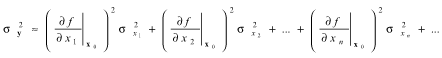
For x is a set of design variables or parameters or factors. Approximation of s_y is “good” when y is approximately linear in a 2s– -3s neighborhood of x₀.

Robust design can be obtained by minimizing the performance variability, i.e., s²_y. This can be done by either minimizing the sensitivities, i.e., derivatives of f(x), or minimizing variability of design variables, i.e., s_x1, …, s_xn. Optimal design can be obtained by selecting nominal values of other certain design variables, i.e., x₁, …, x_n, to bring the system performance mean to its target. Minimizing design variables or parameter sigma by improving process capability is mainly part of DMAIC Six Sigma.Minimizing the sensitivities by selecting nominal values of design variables,i.e., x₁, …, x_n, is mainly part of DFSS.

Following the mean-variance model above and applying vector loop technique for stack-up analysis, the transfer function of the clearance and its variance can be derived as follows:

Clr. = d – c – 2(b + a/tan[q]) and s²(Clr.) = s²(d) + s²(c) + 4s²(b) + 4s²(a)/tan²(q) +4a² Secan²(q)/ tan²(q)

Step 4. Finding Optimal and Robust Design

Finding the best setting of certain design variables can minimize performance variability and others than already-chosen design variables can adjust performance mean to target. This kind of approach was originated by Dr. Genichi Taguchi.

Design of Experiments – Choosing design space and number of levels or settings of the design variables in experimental design need to include engineering and production knowledge. The baseline and benchmark values also should be considered in choosing the design space. To explore high order interaction effect or the nonlinearity relationship between a specific design variable and its system performance, there is a need to choose more levels of that variable as for variables a and theta. The standard deviation of each design variable should be obtained from a stable and under-control process.

Then an appropriate experiment matrix is created. With analytical expressions of the system performance and its variation in hand, the outputs of the experiment are obvious. In this case, a full factorial design generated from DOE Pro XL or Minitab is applied and then the values of Clr. and its standard deviation using their explicit formulas in MS Excel are generated.

Global Sensitivity Analysis – Having generated experimental output, the next step is to analyze the sensitivity of Clr. and its standard deviation in relation to the design variables on their chosen design space. Global sensitivity analysis is very important to rank the importance of the design variables, especially in sequential design of experiments to identify the effective design variables included in design. Analysis of variance (ANOVA) is one tool to get the global sensitivity of the system performance, as shown in the table below.

Analysis of Variance (ANOVA)
Clearance						Standard Deviation (Clearance)
Source	SS	df	MS	P	% Contrib.	Source	SS	df	MS	P	% Contrib.
a	10.7000	3	3.6000	0.0	00.96	a	638.400	3	212.8	0.0	86.63
b	360.0000	2	180.0000	0.0	32.39	b	0.000	2	0.0	1.0	00.00
c	360.0000	2	180.0000	0.0	32.39	c	0.000	2	0.0	1.0	00.00
d	360.0000	2	180.0000	0.0	32.39	d	0.000	2	0.0	1.0	00.00
theta	17.2000	4	4.3000	0.0	01.55	theta	82.100	4	20.5	0.0	11.14
AE	3.4487	12	0.2874	0.0	00.31	AE	16.500	12	1.4	0.0	02.24
Error	0.0000	514	0.0000		00.00	Error	0.000	514	0.0		00.00
Total	1111.3980	539				Total	737.013	539

The ANOVA table shows that a and theta have about 98 percent influence to minimize performance variability (StDev[Clr.]) and b, c and d have about 97 percent influence to optimize the performance mean (Clr.). Small interaction between a and theta occurs to both of the performance variability and mean.

Graphical Approach – The direction to find the best settings of the variables are shown through the main effect and interaction plots of the experimental results as shown in Figure 3, obtained from Minitab.

The plots indicate that decreasing a and increasing theta will minimize performance variability, and selecting settings for b, c and d will adjust the performance mean to target, but they do not affect the performance variability. This approach is called graphical approach. (In order to optimize the baseline design to its target, without considering robustness, it would be intuitive to increase a and decrease theta. This would get an optimal solution, but the solution would not necessarily be robust.

Mathematical Programming Approach – Graphical approach cannot provide an easy way to find optimal and robust solutions when there are multiple performances or the interactions among the design variable are significant. In such situations, what needs to be applied is a mathematical programming approach, e.g., dual response optimization for performance mean and variability problems, or desirability function method-like approaches for multiple performances.

Dual response optimization is to minimize StDev(Clr.) subject to clearance on target and the design variables in design space. This can be implemented by using add-in MS Excel Solver.

In many cases each performance has different magnitudes. One way to normalize each performance into values between 0 and 1 is to implement desirability function method. Optimizing clearance is to find its best nominal values. Optimizing (Clr.) is to minimize (Clr.).

Once performances are converted into individual desirability that has values between 0 and 1, weighted geometric mean aggregate methods may be used to combine the individual desirability. Finally, optimizing the aggregate value is equivalently to optimizing each individual performance, i.e., clearance and its standard deviation. Multiple objective optimizations will generally end up with what are called Pareto optimal solutions. These solutions are suitable to satisfy a family of products whose performance targets are various.

The baseline design results compared to the optimal and robust design results using Minitab Optimizer which is based on desirability function method are shown in Figure 4.

The robust design gives performance mean close to the target, i.e., 0.8 with the performance variability only 0.83. The design is robust more than 3.5 times than the baseline design. Moreover, the robust design relaxes the theta tolerance from StDev = 4 to StDev = 5.

Guide for Manufacturing and Quality Process – From the equation of the variance of y for a point x0 above, the local sensitivity of the design variables is defined as:

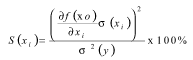
The local sensitivity of the robust design using Crystal Ball v.7 is given in Figure 5. This shows that roller distance (c) and door height (d) are the most sensitive variables in relation to the system performance mean, as their influence on clearance is as much as 80 percent. Track length (a) and roller angle (theta) are the only influential variables to the system performance variability. Those results can be applied as early identification to allow, e.g., quality assurance people to focus on variables c and d in their control process, and manufacturing or supplier people to plan for variables c and d in their facility and tooling up front.

Robust design also identifies that variables a and theta have minimum influence on optimal performance mean. Therefore, the tolerance of both variables can be relaxed without loosing significantly the optimal and robust design.

Monte Carlo Simulation – In the case, with the explicit transfer functions of clearance and its standard deviation, the distribution of the design variables is known, i.e., normal. With this information, Monte Carlo simulation software can be used to find the best setting of the design variables for robust design.

Step 5. Tolerance Design

The process shown above can be repeated to get the optimal tolerance for each design variable. This is about how to economically allocate the performance tolerance to the tolerance of the controllable and uncontrollable variables. The algorithm is to fix the design variables at values to get the optimal and robust design and then to change the deviation of the variables.

Conclusions: The Values of DFSS

• The ultimate goal of DFSS is to have products or processes which are insensitive to the sources of variation that inhibit their intended function, and thus to improve customer satisfaction.
• DFSS defines the relationship between the product or process performances and their controllable and uncontrollable variables. This provides a guide to the product development process to avoid over or under designs, drive focus on design essentials, shorten the product development cycle and reduce cost.
• DFSS provides early identification of factors critical to the customer (characteristics) that allows manufacturing to plan for those factors in its facility and tooling up front. This provides a guide to manufacturing and quality processes. Thus, DFSS speeds up delivery, improves quality and prevents cost of poor quality.
• Once the functional subsystem is completely understood, DFSS provides a quality opportunity with replication of the methodologies on other applications. Thus, DFSS improves organizational design knowledge.