
In the Analyze phase of a DMAIC (Define, Measure, Analyze, Improve, Control) Six Sigma project, potential root causes of variations and defects are identified and validated. Various data analysis tools are used for exploratory and confirmatory studies. Descriptive and graphical techniques help with understanding the nature of data and visualizing potential relationships. Statistical analysis techniques, such as hypothesis testing and regression, are used to validate the root causes.
While one of the statistical methods widely used in the Analyze phase is regression analysis, there are situations that warrant the use of other nonparametric methods. Violation of the basic assumptions of normally and independently distributed residuals, and the presence of nonlinear relationships, are the most common situations where using a nonparametric method, such as a classification and regression tree (CART), is more appropriate. In addition, CART can be appropriate in service industries such as banking and healthcare where many potential causes of variation and defects are categorical in nature (e.g., geographical locations, products, channels, partners). The problem with using regression or generalized linear models (GLM) in such cases is that a lot of dummy variables make it difficult to interpret the results. CART is a useful nonparametric technique that can be used to explain a continuous or categorical dependent variable in terms of multiple independent variables. The independent variables can be continuous or categorical. CART employs a partitioning approach generally known as “divide and conquer.”
How CART Works
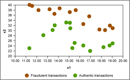
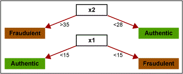
Assume there is a set of credit card transactions labeled as fraudulent or authentic. There are two attributes of each transaction: amount (of transaction) and age of customer. Figure 1 displays an example map of fraudulent and authentic transactions.
The CART algorithm works to find the independent variable that creates the best homogeneous group when splitting the data. For a classification problem where the response variable is categorical, this is decided by calculating the information gained based upon the entropy resulting from the split. For numeric response, homogeneity is measured by statistics such as standard deviation or variance. (For more information on this please refer to Machine Learning with R by Brett Lantz.)
Two important parameters of the CART technique are the minimum split criterion and the complexity parameter (Cp). The minimum split criterion is the minimum number of records that must be present in a node before a split can be attempted. This has to be specified at the outset. Cp is a complexity parameter that avoids splitting those nodes that are obviously not worthwhile. Another way to consider these parameters is that the Cp value is determined after “growing the tree” and the optimal value is used to “prune the tree.”
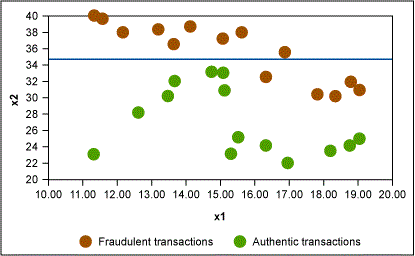
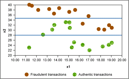
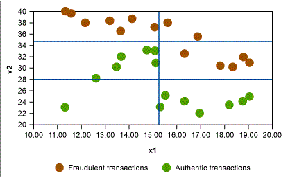
In this example, Figure 2 shows that the first rule formed is x2 > 35 → fraudulent transaction. Similarly, other rules are formed as shown in Figures 3 and 4.
In this way, the CART algorithm keeps dividing the data set until each “leaf” node is left with the minimum number of records as specified by minimum split criterion. This results in a tree-like structure as shown in Figure 5. The Cp value is then plotted against various levels of the tree and the optimum value is used to prune the tree.
Application of CART
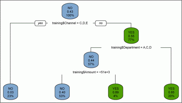
The following example contains a hypothetical dataset of 600 dispatch transactions of a bank.

The dependent variable is the attribute “defective,” which is a categorical variable with two classes (yes and no). Each transaction is labeled either “yes” or “no” based on whether there is any printing error in the deliverable. The independent variables are “amount,” “channel,” “service type,” “customer category” and “department involved.” The first step in applying any analytical method is to explore the data using descriptive statistics. Assume that in exploring the data all of the independent variables seem to have a significant relationship with the dependent variable. In order to carry out the CART analysis, the dataset is randomly split into two sets, the training and testing sets. Nonparametric studies are not based upon theoretical-probability distributions; it is widely accepted practice to build a model on one set of data and test it on another. This helps in ascertaining the accuracy of the model on unknown future records.
The CART model is used to find out the relationship among defective transactions and “amount,” “channel,” “service type,” “customer category” and “department involved.” After building the model, the Cp value is checked across the levels of tree to find out the optimum level at which the relative error is minimum. The optimum Cp value is then used to prune the tree.
Post-pruning, the “final” tree can be created as shown in Figure 8. The model can also be validated against test data to ascertain its accuracy.
Advantages of CART
As with other nonparametric techniques, CART does not require any assumptions for underlying distributions. It is easy to use and can quickly provide valuable insights into massive amounts of data. These insights can be further used to drill down to a particular cause and find effective, quick solutions. The solution is easily interpretable, intuitive and can be verified with existing data; it is a good way to present solutions to management.
Limitations of CART
Like any technique, CART also has limitations to take into account before doing the analysis and making any decisions. The biggest limitation is the fact that it is a nonparametric technique; it is not recommended to make any generalization on the underlying phenomenon based upon the results observed. Although the rules obtained through the analysis can be tested on new data, it must be remembered that the model is built based upon the sample without making any inference about the underlying probability distribution. In addition to this, another limitation of CART is that the tree becomes quite complex after seven or eight layers. Interpreting the results in this situation is not intuitive.
Conclusion
CART can be used efficiently to assess massive datasets and can provide quick solutions in the Analyze phase of DMAIC. CART can be one of the quickest and most effective tools in the bag of any process improvement practitioner. CART should not, however, replace corresponding parametric techniques. The latter is always more powerful in terms of explaining any phenomenon owing to the nature of underlying distribution.