Basic terminologies of time series and forecasting can be difficult to understand. There are four basic learning points:
- The definition of forecasting
- Forecasting as a business and communicative process (not a statistical tool)
- General definitions used in forecasting (regardless of statistical tool)
- The statistical/mathematical techniques
Becoming Aware of the Broad View of Forecasting: Overview – Applications and Basic Steps
Forecasting is the prediction of future events and conditions and is a key element in service organizations, especially banks, for management decision-making. There are typically two types of events: 1) uncontrollable external events – originating with the national economy, governments, customers and competitors and 2) controllable internal events (e.g., marketing, legal, risk, new product decisions) within the firm.
The need for forecasting stems from the time lag between awareness of an impending event or need and the occurrence of that event. Organizations constantly try to predict economic events and their impact.
The following are a few applications for forecasting modules:
- Forecasting utilization rates for credit cards: build a model based on historical data and use the model to score a current credit card portfolio to determine utilization rates.
- Model loss rates of a group of home equity lines of credit as a function of time.
- An independent system operator, organized for monitoring the electrical grid, has a need to predict electrical usage – the volatility of the daily usage can be thought of as a blend of day-ahead-market volatility and monthly volatility, where the month can be one or more months forward.
There are some basic steps for creating a forecast:
- Define the problem. How will the forecasts be used, who needs the forecast and what is the voice of the customer (VOC)?
- Gather the necessary information by obtaining historical (mathematical) data and utilizing the accumulated judgment and expertise of key personnel.
- Determine what graphical plots will best benefit management and design a preliminary analysis. Include descriptive statistics.
- Choose and fit models by using and evaluating a forecast model for decision making. Forecast errors and management response.
Forecasting System
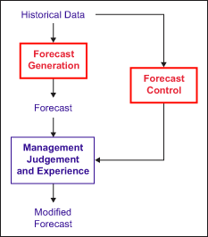
A forecasting system consists of two primary functions: forecast generation and forecast control. Forecast generation includes acquiring data to revise the forecasting model, producing a statistical forecast and presenting results to the user. Forecast control involves monitoring the forecasting process to detect out-of-control conditions and identifying opportunities to improve forecasting performance. Figure 1 shows a visualization of a forecasting system and process.

Forecasting Terminology
There are a number of common terms when discussing forecasting models:
- Point forecast: a single number that represents the best prediction (or guess)
- Prediction interval forecast: an interval (or range) of numbers that the actual value will be contained within – provides the “best” and “worst” case estimates of forecasts
- Out-of-sample (ex-ante forecasts), cross-sectional and time series data: refers to data used to validate the forecasting model and compares forecasted values to the out-of-sample data. Conversely, in-sample data refers to the data used to construct the model. Users should fit the model to the in-sample data.
- Out-of-sample data selection: data sets used to validate forecasts can be obtained in several ways:
- Hold out x percent of most recent (rule of thumb is 10 percent) – usually for longitudinal data
- Hold out x percent but randomly throughout the entire data set – usually for cross-sectional data
- Use all data and wait for future values:
- Cross-sectional data (regression techniques) where all observations are from the same time
- Time series data (signal/noise techniques): a chronological sequence of observations
Forecasting Measures of Errors
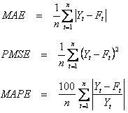
In any forecasting, it is the accuracy – or “goodness of fit” – of future forecast(s) that is most important. There are three commonly used statistical measures used in forecasting: 1) mean absolute percentage error (MAPE), 2) mean absolute deviation error (MAD or MADeviation) and 3) predicted/mean squared deviation error (PMSE or MSDeviation).
If Yt is the observed value at period t and Ft is the forecasted value at period t

| Table 1: Examples of Forecast Error Measures | |||||
| Period | Observed | Forecast | Abs Error | % Abs Error | Deviation2 |
| 1 | 138 | 150.25 | 12.25 | 8.9 | 150.06 |
| 2 | 136 | 139.50 | 3.5 | 2.6 | 12.25 |
| 3 | 152 | 157.25 | 5.25 | 3.5 | 27.56 |
| 4 | 127 | 143.50 | 16.5 | 13.0 | 272.25 |
| 5 | 151 | 138.00 | 13 | 8.6 | 169.00 |
| 6 | 130 | 127.50 | 2.5 | 1.9 | 6.25 |
| 7 | 119 | 138.25 | 19.25 | 16.2 | 370.56 |
| 8 | 153 | 141.50 | 11.5 | 7.5 | 132.25 |
|
Totals |
83.75 | 62.12% | 1140.19 | ||

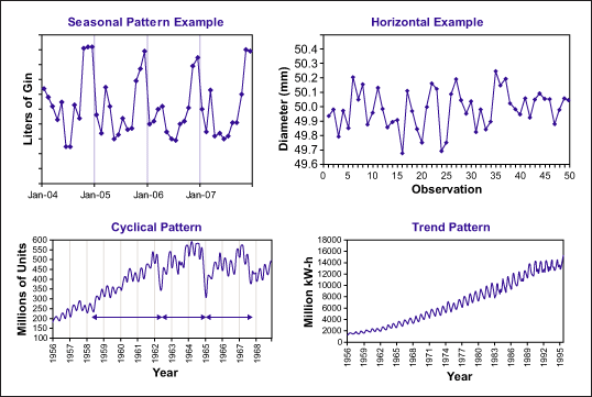
- Time series patterns: common patterns are called horizontal (stationary), seasonal, cyclical, and trends
- Adjustments by number of days: some of the variation in a time series may be due to variation in the number of days (from 28 to 31) per month (e.g., trading days). Use the following formula to make this adjustment before doing any forecasting.

Adjustments by inflation: a cause of variation that affects time series is the effect of inflation.When forecasting the price of a new SUV (or car), it is essential to take into account the effect of inflation, as a $80,000 SUV this year is not the same as a $80,000 SUV 10 years ago. By using the equivalent value in the year 2007, for example, the data are then directly comparable and forecasts will have one less source of variation.
- Adjustments by population: population change is another source of variation. When forecasting the number of public transport users in a city, it is preferable to take into consideration the effect of population changes. In this case, the data fluctuates based on the total number of people in the city. Rather than forecasting the total number of public transport users, it will be more accurate to forecast the proportion of people who are public transport users.
- Stationarity: this refers to the stability of a process’s mean and variance across time. If there is no growth or decline in the data, the process is said to be stationary in the mean. If there is no obvious change in the variance across time, the process is said to be stationary in the variance.
- Autocorrelation: this is a measure of how consecutive observations are related. The observation Yt-1 is described as lagged by 1 period. Similarly, it is possible to compare observations lagged by two periods, three periods, etc.
Forecasting Methods – Trade-Offs
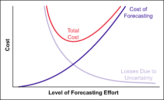
There are many factors to consider when choosing a forecast method. Two major considerations are cost versus risk.

Summary
“Prediction is very difficult, especially if it’s about the future.”
–Nils Bohr, Nobel laureate in Physics
This quote serves as a warning of the importance of testing a forecasting model out-of-sample. It is often easy to find a model that fits the past data well. It is quite another matter to find a model that correctly identifies those features of the past data that will be replicated in the future. Do not create a model to be an exact replica of reality. Create a model because it is quick and easy and guides toward reality. A model also emphasizes the complexity and unreliability of predictions.