In this two-part article, uncertainty quantification (UQ) is explained. Last week, in Part 1, we learned the basics of UQ and how UQ works with Six Sigma. This week, Part 2 is a case study looking at UQ in action.
UQ Case Study: Redesign of a Bracket Fatigue Model
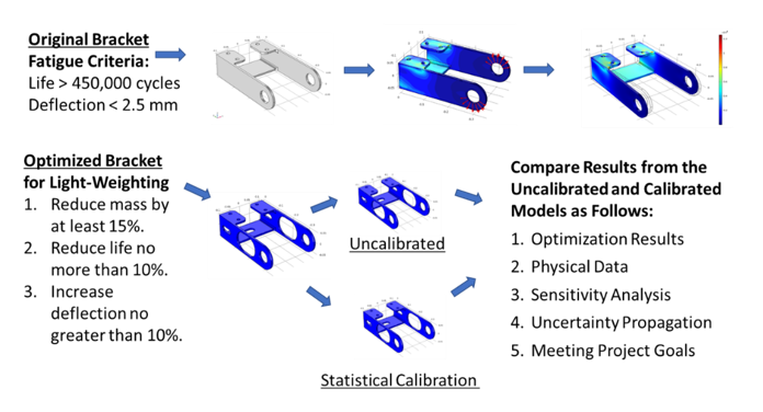
This case study will show how UQ techniques can be used to perform robust risk estimation, identify key drivers of manufacturing variability and gather more information for critical decisions. The goal of this example is to reduce a bracket’s mass by 15 percent but not affect the fatigue cycle life or the deflection any greater than 10 percent of the original bracket criteria.
As shown in Figure 1, the original bracket has the fatigue life of more than 450,000 cycles with a deflection of less than 2.5 mm. To find the optimal bracket mass, two emulators will be built with one emulator being calibrated. Statistical calibration is used to correct for bias in the simulation results against a set of experimental test points. To compare the two models, the emulators will undergo multiple analyses including optimization, sensitivity analysis and uncertainty propagation.
Analysis Setup
The model inputs are the geometric parameters of the mass-reducing slots in the bracket and the applied loads and mechanical properties of the bracket material. The model responses of interest are the mass (kg), fatigue life (N) and displacement (mm).
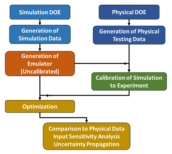
As shown in Figure 2, the analysis starts with developing a simultion and physical testing design of experiments (DOE). The emulator for the uncalibrated model is built using the DOE inputs and the simulation outputs, and the emulator for the calibrated model incorporates data from both the physical and simlation datasets. Both emulators undergo a validation process, which tells the analyst the error in the emulators when compared to the physics-based simulations.
Once the emulators have met the accuracy criteria, they will undergo optimization, minimizing mass with the constraints for fatigue life and displacement. Then, sensitivity analysis is used to locate key input variables to inform future design decisions and constraints. Finally, uncertainty propagation about the optimal point is performed to assess the robustness of the design to various geometric and material uncertainties. The results of the emulators will be compared at each step.
Results of a Bracket Fatigue Model
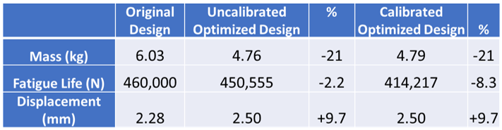
After both emulators are built and validated, the team performed an optimization to maximize the mass with the constraints on the fatigue life and displacement. Figure 3 shows the results of the two optimizations compared to the original bracket design. Both optimizations met the criteria of mass reduction, fatigue life and displacement.
Since the two emulators did not find the same optima, this raises questions like the following:
- Are the optima from the calibrated emulator more accurate and robust than the uncalibrated emulator?
- Are key design parameters significantly affected by the calibration process?
- Will variations in manufacturing influence key design requirements?
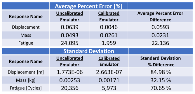
To answer these questions, multiple iterations of the emulators were run, and predictions were made. Figure 4 shows the average percent error and standard deviation of the two emulators. The calibrated model had a smaller average percent error and standard deviation than the uncalibrated model for all the simulation responses. This is an expectation of the calibration process in that it tunes the model to produce results that are more realistic.
To understand which inputs have the greatest influence on fatigue life, a sensitivity analysis was performed for both emulators. As shown in Figure 5, the d2 slot governs the fatigue cycles to failure response for both emulators. In addition, the sensitivity analysis for the two emulators have the same parameter rankings for the fatigue life response.
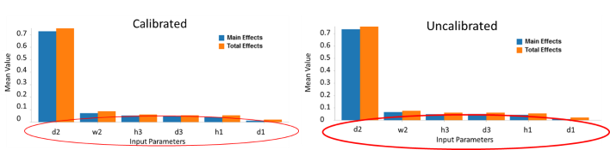
Both results are important for this analysis.
- Knowing that the d2 parameter controls fatigue life means that this is the parameter to adjust and increase the fatigue life. Moreover, the geometry of the d2 slot may require more stringent tolerances when fabricated to maintain the fatigue life target.
- If the ranking of the slot parameters were different, it would imply that the original physics may not be correct. Since this is not the case, the equivalent input sensitivity rankings support model validation of the simulation.
After performing the sensitivity analysis, the next step is to determine the robustness of the model results by propagating uncertainty through the optimal point of each emulator. Propagating uncertainty through the emulator is a way to examine the impact of fatigue life on variations in the geometric slots from manufacturing. In this scenario, a ±5 percent variation was assumed on the emulator inputs to represent typical variations found in manufacturing.
Once the uncertainty propagation is performed, the results take the form of a histogram of the variation about the optima. Figure 6 shows the histograms of fatigue life for both emulators. The histogram of the uncalibrated emulator has a one percent chance of not meeting the fatigue life criteria from variations in manufacturing whereas the histogram of the calibrated emulator has a 47 percent chance of not meeting the criteria.
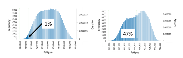
In terms of decision-making, if the analysis was only made using the uncalibrated emulator, the analyst would likely proceed with this optimal bracket design since there is only a small chance of not meeting the target fatigue life. If the analysis included calibrating the emulator, however, the risk of going forward with this design would include a high probability of not meeting the target fatigue life.
Summary
The bracket fatigue case study highlights the value of three UQ methodologies:
- Sensitivity analysis
- Statistical calibration
- Uncertainty propagation
The sensitivity analysis identified the key drivers in the manufacturing variability and supported model validation of the bracket simulation. By performing statistical calibration, the simulation results are more realistic and, thus, reduced the risk of poor decision-making.
Finally, performing uncertainty propagation with the calibrated model assessed the impact of manufacturing variations to fatigue performance metrics. By calibrating the model, a significant amount of time and resources were likely saved, and in terms of justifying the use of UQ, these items are measurable. Moreover, the analyst knows which parameter to adjust to meet the fatigue life target for the next design iteration.
*Note: All images courtesy of SmartUQ.