
Article authors, participants in discussion forums and even software documentation claim that any data and especially time-sequenced data are useful only if they are homogeneous – that is, only if they display control chart stability (CCS).1,2,3,4 According to one quality control expert, Donald J. Wheeler, when out-of-control signals occur, “all of our computations, and all of our conclusions, are questionable.”1
Fortunately, CCS is not always needed for either predictions or baseline estimates for process improvement. By recognizing the limitations of CCS, better prediction methods can be used that require less effort.
Predictions
There are two types of predictions: interpolation and extrapolation. Interpolation is predicting or estimating between known quantities, while extrapolation is predicting or estimating beyond the data. For example, if data exists for the odd-numbered years from 2001 to 2011, interpolation predicts the even-numbered years, while extrapolation predicts the years before 2000 or the years after 2013. People have successfully interpolated and extrapolated for centuries prior to the invention of control charts (e.g., lunar eclipses and phases). Control charts do have a role in predictions, but that role is limited.
Limitation: Interpolation When Stable Is No Better Than When Unstable
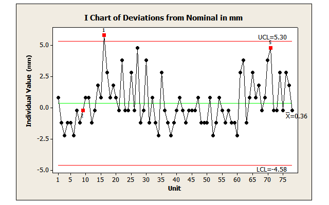
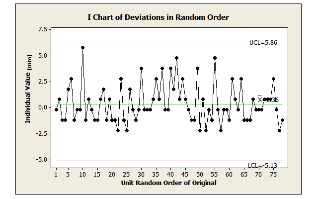
CCS allows for a prediction only within a range shown by historical results, not an exact value. No more should be expected when lacking CCS. Figure 1 shows deviations from nominal diameter for 78 pipes lacking CCS. However, the same is true if the data had occurred as in Figure 2, showing CCS.
Solution
The reason has nothing to do with stability. It can, in fact, be arbitrary. If the average of continuous data is taken to one more significant digit than the original data, it will not equal any of the values in the data set. As another example, consider a case in which the average is not an integer, but all the possible values of a count distribution are integers – the average of a fair die with sides numbered 1 through 6 is 3.5, which is not any of the actual choices. Requiring stability adds nothing but extra work in this case.
When all of the data exists, do not interpolate – there’s no need to estimate because all of the data is known. Instead, characterizations of the existing data can be made. (For example, how many pipes had deviations > 2.5 mm? Fourteen.)
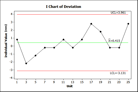
When all of the data is not available, CCS does not mean that the missing data is consistent with the existing data. Figure 3 shows an I-chart exhibiting CCS using only every other pipe of the first 25. Using CCS, it can be predicted that each odd-numbered pipe deviates from nominal from -3.131 mm to 3.961 mm. Yet, pipe 16, one of the missing data points to be estimated, had a deviation >5.0 mm (see Figure 1).
Using the minimum and maximum of past results is just as good a predictor without requiring CCS. When making predictions requiring CCS, as soon as the chart shows instability the predictions must stop. The process must stabilize again before being able to make predictions again. Using the minimum and maximum, however, allows for the altering of the range or margin of error.
Limitation: Inaccuracy in Extrapolating Based on Stability Alone
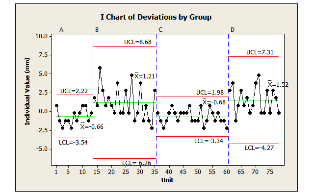
CCS implies that there can always be a prediction made from stable processes within a margin of error defined as the control limits of the chart. In Figure 4, each CCS period has its margin of error for predicting (e.g., -3.54 mm to 2.22 mm from the first 13 pipes).
CCS does not, however, specify how far into the future the prediction applies: a few seconds, months or years? How many more pipes are expected to have deviations within this range? Three other limitations to requiring CCS include the following:
- As soon as instability occurs, prediction stops.
- Only future extrapolation is allowed, not past extrapolation.
- Some calculated limits cannot occur in practice.
Thus, each CCS period inaccurately predicts when instability occurs and can only predict for a limited time. The first CCS period (pipes 1 through 13) incorrectly predicts 7 of the next 22 (32 percent) results and 14 of the next 65 (22 percent) results, while the third CCS period (pipes 36 through 60) incorrectly predicts 7 of the next 18 (39 percent) results.
Solution
Predictions can always be made using the maximum value in the data set as the upper prediction limit (UPL) and the minimum value as the lower prediction limit (LPL). The minimum-maximum method accurately predicts for longer periods into the future with only two points – even when the process is unstable. These values will not necessarily equal the lower and upper control limits, especially when the chart does not display stability.
For example, for the first 13 pipes, using LPL = minimum data point = -2.2 mm and UPL = maximum data point = 0.8 mm, results in an incorrect prediction for the pipe 14, which has a value of 1.8 mm. By changing UPL to 1.8, the deviation of pipe 15, 0.8 mm, can be correctly predicted but not the 5.8 mm value for pipe 16. By changing UPL to 5.8 mm, 100 percent of the next 62 deviations can be correctly predicted. If we the UPL is not changed when the limits are exceeded, then the level of confidence of correct predictions drops as there is data that shows the limits are not always predictive.
Does minimum-maximum arbitrarily widen the limits to increase accuracy without regard to utility? Control chart limits do not inherently provide predictive utility. A process can be stable with very wide limits.
For example, using pipes 14 through 35, the control limits are -6.26 mm and 8.68 mm (Figure 4). These limits correctly predict all subsequent deviations. If deviations had occurred as in Figure 2 (randomly reordering all the data to show CCS), the control limits are -5.13 mm and 5.86 mm. In each case, the CCS limits are wider than the minimum-maximum limits of -2.2 mm to 5.8 mm.
Also, control chart limits can have values that cannot occur in practice (e.g., negative values for dimensions or counts, and fractions for counts). The minimum-maximum approach cannot.
Limitation: Falsely Assuming CCS with Samples
When all the data for a period is used, CCS can identify special-cause variation signals except when a sample of rational subgroups is used. Typically, during the entire period covered by the data, the process is actually unstable due to its low power to detect instability.
Proponents of CCS explain that it is not necessary to identify all instability. If some instability is okay, then even unstable processes are predictable. If no instability is acceptable, then CCS has limited applicability.
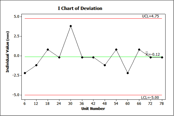
For example, sampling every sixth pipe displays CCS (Figure 5), indicating the data are meaningful and useful for predicting future deviations to be from -5.00 mm to 4.75 mm. But using all 78 deviations shows instability (Figure 1), contradicting this conclusion. (Note that the CCS limits are wider than the minimum-maximum limits of -2.2 mm and 5.8 mm.)
Solution
To use CCS with samples, check for actual stability for the entire period to avoid falsely assuming CCS. This requires extra effort and will work only if all the data shows CCS. The minimum-maximum approach universally applies whether stable or not, without values that cannot occur, and often with narrower limits.
Limitation: Requiring CCS Is Misguided
To improve predictions we want to advance from guesswork to understanding causation.
CCS predictions are no more than guesses based on past patterns. The same is true of minimum-maximum and other pattern-based methods (e.g., stock prices based on past cyclical patterns). CCS applies only when the process is stable and cannot predict when the process will be unstable or what the result will be when it is unstable. Some processes should be stable, others should not (e.g., processes monitoring desirable growth). CCS does not apply to the latter processes.
Solution
There are two ways to make more accurate predictions with smaller error margins: using correlation models or causal relationships (e.g., scientific laws). Based on causes, predictions can be made without requiring CCS and can predict specific values with less error. Meteorologists make predictions daily, forecasting one to 10 days in advance – not through the use of control charts, but by understanding the causes of weather and temperature. They predict hourly future temperatures even when it may be out of control (e.g., sudden drop due to a cold front).
Children learn to predict how much effort they need to toss a ball a certain distance without using control charts. Even if a control chart of their distances showed lack of control, they can still predict scientifically – but not by using CCS.
Figure 6 shows data with a lack of CCS. CCS proponents would claim that the process is unpredictable. However, this data comes from an actual exercise used to illustrate the benefits of designed experiments and regression analysis. The data represents the distance a puck traveled using a slingshot. Regression analysis showed a linear relationship between force and distance traveled. Participants in the exercise accurately predict how far the puck will travel given the force used for various forces and in any order.
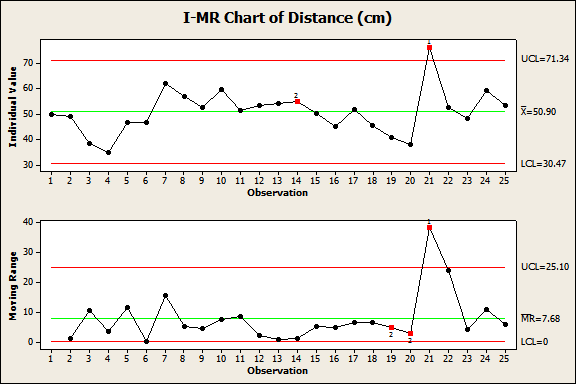
Figure 7 shows the data ordered by four ranges of force with each range displaying CCS. Using CCS, only predictions within the margin of error for that stage are permitted. By understanding and controlling the causes, predictions are possible without CCS.
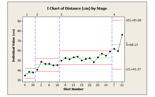
Figure 7: Distances Traveled By Stages Representing Ranges of Force
Process Improvement
Before embarking on process improvement, it’s typical to determine a baseline of performance. After a process change, a new baseline is calculated. These two baselines are compared to confirm the change was successful. CCS is unnecessary.
Limitation: Lack of Universality
CCS is not applicable for determining baselines or making comparisons when the process displays instability. To use CCS, extra effort is needed to make the process stable. If the purpose, however, is to determine what happened during a period or to compare two periods, changing the process to stabilize it no longer explains what happened during those periods.
Solution
A baseline simply describes a static population. There are two easy ways of describing a baseline: 1) all the data from the period of interest with descriptive statistics, or 2) random sampling using inferential statistics.
Consider the example of deviations from the nominal pipe diameter when all of the data for the period of interest is available. Regardless of the order, the mean deviation and baseline is 0.36 mm, whether with CCS (Figure 2) or without CSS (Figure 1).
If it is not desirable to use all of the data, take a random sample to calculate a point or confidence interval estimate, or even to test statistically. The validity of random samples can be verified through simulation. Construct, for example, 95 percent confidence intervals, for the mean of the 1,000 samples without replacement from the data of size 2 < n < 78. (Other quantities, 90 percent or 99 percent, will also work.) Construct x percent confidence intervals for the mean of the 1,000 samples. Determine the percent that includes the mean 0.36 mm. That will equal approximately x percent. This isthe definition of a confidence interval. An x percent confidence interval of size n means that x percent of all possible confidence intervals of size n will include what is being estimated. If it is the true mean of 10, then 95 percent of all 95 percent confidence intervals will include 10.
Limitation: Falsely Assuming CCS with Samples
As with predictions, when not all data for the period of interest is used, CCS may be falsely assumed. Sampling every sixth pipe, the control chart appears stable (Figure 5), wrongly implying the entire period covered by the 78 pipes was stable. Using this sample to determine a baseline contradicts the CCS requirement.
Solution
Ignore whether the control chart is stable. Baselines are for specific periods and not the entire life of a process. Select the period or periods of interest. Use all the data from the selected timeframe or take a random sample – not rational subgroups.
Limitation: Illogical Conclusions
Requiring CCS for all comparisons results in illogical conclusions, such as the following:
- You buy a case of 24 bottles of your favorite beverage. Noticing one is empty, you complain to the vendor. He replies, “Maybe it is empty, maybe it is not. If the process that produced them was not in control, we do not know if it is empty.”
- Your 5-year-old daughter asks how much taller is she now than last year. You reply, “Unfortunately, because growth is a process that is out of control (upward trend), I cannot compare or use any period as a baseline. The measurements are useless.”
- You wagered on the losing team of a baseball game that went 18 innings and had a final score of 1-0. You tell your bookie, “I still do not know who won because a control chart of the team that scored the winning run shows it is out of control. So, I cannot use that run as a baseline to compare.”
Solution
Do not check for stability. Clearly, valid and correct comparisons can be made without ever knowing whether the results came from a stable process – and without using control charts. The individuals above know that 1 out of 24 bottles is empty, the daughter is taller, and the bet is lost.
Why Control Chart Stability Has Limitations
There are several reasons for CCS limitations and contradictions.
Confusing Enumerative with Analytic
Baselines are enumerative statistics; they are answers to the questions “What?” or “How much?”7 They are not answers to the analytic question “Why?” even when doing process improvement. Predicting simply because a control chart displays stability does not tell us why this average or these individuals result. Knowing the causal relationships and existing conditions does tell us why the result did, or will, occur.
Assuming That Appearing Stable = Stable
Figure 5 shows that when all of the data is not available (e.g., with rational subgroups), a lack of special cause variation or instability does not mean the process was actually stable. In many cases, it will not be – either with small or large unstable variations. This contradicts the premise that only data from stable processes is useful whether for predicting or estimating baselines.
Assuming That Stability = One Process or Cause System
If Figure 4 indicates that there are two or more processes defined as distinct cause systems, then Figures 2 and 3 show that even when a process appears stable, it does not mean that there is only one cause system.
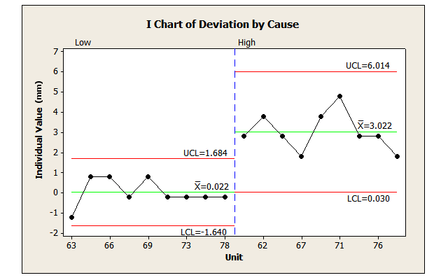
How many cause systems appear in the last 18 deviations (Figure 2)? In the actual order, that cannot be determined with a control chart. There could be two causes: (low) average of 0 with a range of -1.2 mm to 0.8 mm and (high) average of 3 with a range of 1.8 mm to 4.8 mm. By rearranging the data by cause systems (Figure 8), it appears there are four.
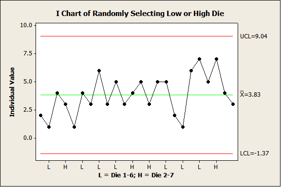
This point can be illustrated by using one die with sides numbered 1 through 6 and another numbered 2 through 7. Assign one side of a coin to the first die and the other side to the second dice. Flip the coin, toss the appropriate die, and then record the result. Repeat for 25 results. Plot the data.
Figure 9 shows one result. How many processes or cause systems? Two, one per die (although that is not apparent in Figure 9 that displays CCS).
Confusing the Question Control Charts Answer
Predictions answer the question “What will X be?” or “What was X?” where X might be an average, count, percent, maximum, minimum, individual value, etc. Requiring CCS changes the question to “Is A the same as before?” When it is not or does not appear stable, control charts cannot say what A is, limiting its utility.
Baselines answer “How much is A?” for specific periods. Baseline comparisons for two specific periods answer “Is A different than B?” Requiring CCS changes these two questions to “Is A the same during the period?” and “Could the difference between A and B be due to a change in the process?” Answers to these questions do not answer the baseline questions.
Conclusion
CCS advocates could contribute more by specifying when and why CCS is applicable rather than always requiring it. In particular, it helps to know what questions CCS does and does not answer. This increases appropriate control chart use.
But CCS is not what allows prediction. As stated by engineer and statistician Walter Shewhart, “The fact that an observed set of values of fraction defective indicates the product to have been controlled up to the present does not prove that we can predict the future course of this phenomenon. We always have to say that this can be done provided the same essential conditions are maintained, and, of course, we never know whether or not they are maintained unless we continue to experiment.”8
Knowing the limitations of CCS and the reasons for them frees process improvement professionals to find and use universal methods that better answer questions with respect to predicting, estimating baselines and improving processes.
The purpose of analytic studies is to learn the causal relationship between the conditions and the desired results. As knowledge increases, the basis for predictions ought to change from patterns to correlations to causalities. The sequence of studies for process improvement is enumerative-analytic-enumerative: enumerative to establish baselines, analytic to find causes.
Baselines never require stability. Knowing how much never explains why.
CCS is popular and heavily promoted because there are benefits to stable processes. A stable process requires less attention. Control charts are useful for monitoring processes that are desired to be stable. Better still would be controlling process to cause the desired effect.
All processes should not be stable all the time. For example, it is good to have children grow taller and retirement funds to grow larger – and that information can be predicted and compared without CCS.
References
1. Wheeler, Donald J., “Why We Keep Having 100-Year Floods,” Quality Digest, June 4, 2013, http://www.qualitydigest.com/inside/quality-insider-column/why-we-keep-having-100-year-floods.html, Accessed November 30, 2013.
2. Stauffer, Rip, “Render Unto Enumerative Studies…,” Quality Digest, July 31, 2013, https://www.qualitydigest.com/inside/quality-insider-column/render-unto-enumerative-studies.html, Accessed November 30, 2013.
3. LinkedIn, iSixSigma Network group, “How do we validate the samples taken would reflect the population parameter? Or how can we assure that we have taken the correct samples in a Six Sigma project?,” April 2013, https://www.linkedin.com/groupItem?view=&gid=42396&type=member&item=228657002&trk=groups_search_item_list-0-b-ttl&goback=%2Egna_42396, Accessed November 30, 2013.
4. Minitab Version 16, “The process should be stable,” in Guidelines for Assistant>Hypothesis Tests>More.
5. Castaneda-Mendez, Kicab, What’s Your Problem?, Taylor & Francis Group, 2013, Chapters 4-5.
6. Shewhart, Walter A., Economic Control of Quality of Manufactured Product, American Society for Quality Control, 1981, p. 19.
7. Deming, W. Edward, “On the Distinction Between Enumerative and Analytic Surveys,” Journal of the American Statistical Association, Vol. 46, 1953, p. 245.
8. Shewhart, Walter A., Economic Control of Quality of Manufactured Product, p. 148.