In any hypothesis test, there are four possible outcomes. The table below illustrates the only possibilities.

Table 1: Possible Outcomes of a Hypothesis Test
Reality	Decisions
Ho is true	Accepting Ho is true; good decision (p = 1 – a or confidence level)	Accepting Ho when it is false; Type II error (p = b)
Ha is true	Rejecting Ho when in fact it is true; Type 1 error (p = a or significance level)	Rejecting Ho that is not true; good decision (p = 1 – b or power of the test)

What should every good hypothesis test ensure? Ideally, it should make the probabilities of both a Type I error and Type II error very small. The probability of a Type I error is denoted as a and the probability of a Type II error is denoted as b.

Understanding a

Recall that in every test, a significance level is set, normally a= 0.05. In other words, that means one is willing to accept a probability of 0.05 of being wrong when rejecting the null hypothesis. This is the a risk that one is willing to take, and setting a at 0.05, or 5 percent, means one is willing to be wrong 5 out of 100 times when one rejects Ho. Hence, once the significance level is set, there is really nothing more that can be done about a.

Understanding b and 1 -b

Suppose the null hypothesis is false. One would want the hypothesis test to reject it all the time. Unfortunately, no test is foolproof, and there will be cases where the null hypothesis is in fact false but the test fails to reject it. In this case, a Type II error would be made. The probability of making a Type II error and b should be as small as possible. Consequently, 1 -b is the probability of rejecting a null hypothesis correctly (because in fact it is false), and this number should be as large as possible.

The Power of the Test

Rejecting a null hypothesis when it is false is what every good hypothesis test should do. Having a high value for 1 -b (near 1.0) means it is a good test, and having a low value (near 0.0) means it is a bad test. Hence, 1 -b is a measure of how good a test is, and it is known as the “power of the test.”

The power of the test is the probability that the test will reject Ho when in fact it is false. Conventionally, a test with a power of 0.8 is considered good.

Statistical Power Analysis

Consider the following when doing a power analysis:

1. What hypothesis test is being used
2. Standardized effect size
3. Sample size
4. Significance level or a
5. Power of the test or 1 – b

The computation of power depends on the test used. One of the simplest examples for power computation is the t-test. Assume that there is a population mean of m = 20 and a sample is collected of n = 44 and that a sample mean of and sample standard deviation of s = 4 are found. Did this sample come from a population of mean = 20 if it is set that a= 0.05?

Ho: m does equal 20
Ha: m does not equal 20
a = 0.05, two-tailed test

The next example is testing an effect size of 2 . Since this is the absolute value, it needs to be standardized into a t-value using the standard error of the mean .

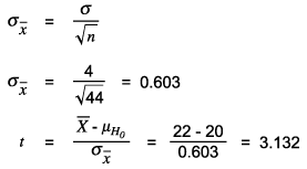
The critical value of t at 0.05 (two-tailed) for DF = 43 is 2.0167 (using spreadsheet software [e.g., Excel], TINV [0.05,43] = 2.0167). Since the t is greater than the critical value, the null hypothesis is rejected. But how powerful was this test?

Computing the Value of 1 -b

The critical value of t at 0.05 (two tailed) for DF = 43 is 2.0167. The following figure illustrates this graphically.

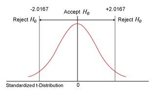
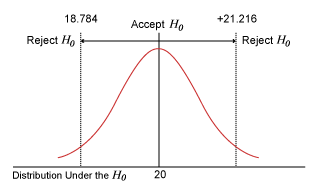
This t = +/-2.0167 equals in the hypothesized distribution = 20 +/- (2.0167) = 20 + 0.603(2.0167) = 21.216 and 20 – 0.603(2.0167) = 18.784.

The next figure shows an alternative distribution of m = 22 and s = 4. This is the original distribution shift by two units to the right.

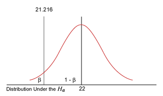
What is the probability of being less than -21.216 in this alternative distribution? That probability is b, accepting Ho when in fact it is false. This is because with any value within that region, in the original probability distribution, one would have accepted Ho. How does one find this b? What is the t value of 21.216 in the alternative distribution?

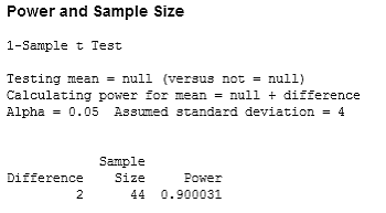
What is the corresponding probability of being less than t = -1.3? From the t-tables, using one-tailed, DF = 43, t = 1.3, one finds 0.10026 (using spreadsheet software TDIST, it is 0.10026). Hence b = 0.10026 and 1 -b = 0.9, which was the power of the test in this example.

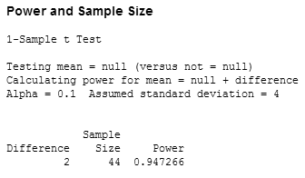
Below is the statistical software output (Minitab) using the same example:

What Influences the Power of the Test?

Three key factors affect the power of the test.

Factor 1

The difference or effect size affects power. If the difference that one was trying to detect was not 2 but 1, the overlap between the original distribution and the alternative distribution would have been greater. Hence, b would increase and 1 -b or power would decrease.

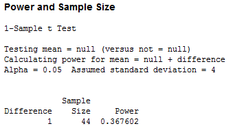
Hence, as effect size increases, power will also increase.

Factor 2

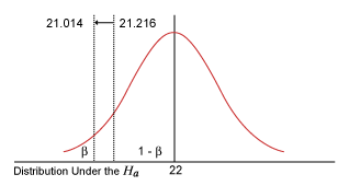
Significance level or a affects power. Imagine in the example using the significance level of 0.1 instead. What would happen?

Table 2: Using a Different Significance Level
Significance Level	DF	Critical t	Value in Original Distribution
0.05	43	2.016692	21.21606538
0.l0	43	1.681071	21.01368563

The critical t would shift from 2.01669 to 1.68. This makes b smaller and 1 – b larger. Hence, as the significance level of the test increases, the power of the test also increases. However, this comes at a high price because a risk also increases.

Factor 3

Sample size affects power. Why? Consider the following equations:

How can t be increased? As t increases, it becomes easier to reject Ho. One way is to increase the numerator or the effect size. As the effect size increases, power also increases. Also, as the denominator or the standard error of the mean (SE mean) decreases, t also will increase, and consequently the power of the test also will increase. How can the denominator be decreased? As the sample size increases, the SE mean decreases. Hence, as sample size increases, t also will increase and the power of the test also will increase.

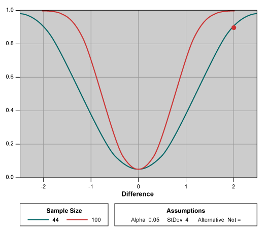
In general, to improve power, really only the sample size can be increased because the significance level is usually fixed by industry (0.05 for Six Sigma) and there is not much that can be done to change the difference trying to be detected.

Since that power of 0.8 is good enough, one can use statistical software to find out what the corresponding sample size is that will be need to be collected prior to hypothesis testing to obtain a good power of test.