
Some Six Sigma practitioners are concerned about the current method used to calculate Z-scores and express process capability. A proposed modification, based on Berryman’s scorecard, may fill the need for a more intuitive and business savvy metric.
The common terminology for describing the capability of a business process is process sigma, or Z-score. Z-scores provide a universal standard performance metric for vastly different processes. According to this standard, a process sigma of 6.0 equates to 3.4 defects per million opportunities (DPMO). This value is obtained by accounting for the fact that any process in control continues to allow for a drift of about 1.5 sigma. The traditional calculation method results in the following Z-scores for error free processes:
- 0 percent error-free yield = negative infinity Z-score
- 50 percent error-free yield = 1.5 Z-score
- 99.99966 percent error-free yield = 6.0 Z-score
- 100 percent error-free yield = positive infinity Z-score
Some Six Sigma practitioners have raised concerns about the current calculation method and the need to develop a more intuitive Z-score. Because a 50 percent error-free yield does not equal a Z-score of zero, the range of Z-scores from negative infinity to positive infinity gives a false sense of symmetry. The asymmetry is due to the belief that any long-term process variability changes by about 1.5 sigma from its short-term variation.
In addition to the asymmetry in the measurement system, there are questions about the appropriateness of using a negative sigma value. While the method and logic used for negative Z-scores is clear, the intuitive meaning of them is not. What does the negative sigma value mean? What is the meaning of a Z-score of zero? As a manager, how should you react to improvements and reward sigma value gains? While the mathematically minded will argue that it is simply a definition, the fact that questions are raised about its appropriateness puts forth a challenge to the Six Sigma community to develop a metric that makes engineering as well as business sense.
The Need for Change
Recently, a Six Sigma team presented their results for a project where the initial process yield was very low, resulting in a low sigma value. A small effort by the project team, however, made a significant change in the sigma score. The management team was excited about the project team’s work. But their excitement was not as high for another project where the team was charged with making an improvement within an already high-performing process. The current Z-score calculation method does not a provide clear reflection of the effort required to improve processes at various levels of initial sigma value.
The data in Table 1 demonstrates that irrespective of initial process performance and due to the symmetry of the bell curve and the current method of calculating Z-scores, the corresponding increment in the sigma score is the same for an equal amount of yield improvement. For example, a process improvement leading to a decrease of 100,000 DPMO from an initial DPMO of 600,000 and from an initial DPMO of 400,000 leads to the same change in sigma score. This does not reflect that improving a process yield when the process is on the very low end of the performance scale is easier than improving the process yield for one that is performing on the high end of the performance scale.
| Table 1: Comparison of Process Performance Improvement Symmetry Toward 50 Percent Yield | ||||||
| Improvement in DPMO | Initial Yield Less Than or Equal to 50 Percent | Final Yield Greater Than or Equal to 50 Percent | ||||
| Initial DPMO | Initial Z-Score | Final Z-Score | Initial DPMO | Initial Z-Score | Final Z-Score | |
| 1.0 | 1,000,000 | negative infinity | -4.753 | 1 | 4.753 | positive infinity |
| 1.0 | 999,999 | -4.753 | -4.611 | 2 | 4.611 | 4.753 |
| 1.0 | 999,996.6 | -4.5 | -4.445 | 3.4 | 4.445 | 4.5 |
| 100,000 | 800,000 | -0.842 | -0.524 | 300,000 | 0.524 | 0.842 |
| 100,000 | 700,000 | -0.524 | -0.253 | 400,000 | -0.253 | 0.524 |
| 100,000 | 600,000 | -0.253 | 0 | 500,000 | 0 | 0.253 |
| 100,000 | 500,000 | 0 | 0.253 | 600,000 | -0.253 | 0 |
This begs the questions: Should practitioners use a metric that is more intuitive in understanding the initial and subsequent change in sigma value? Should the metric account for the relative effort required to achieve the improvement?
Current Method for Calculating Sigma Score
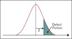
In the current method used to calculate process performance on the sigma scale, the area on a standard normal curve extending from a point some Z-value to the right of center (the mean line) to infinity represents the percent of defects. Figure 1 illustrates this definition of Z-score.
|
|||||
It becomes a bit more confusing once the 1.5 shift in sigma value is considered to account for long- and short-term conversions. Short-term performance is obtained by adding 1.5 to the long-term value. The shift of 1.5 is attributed to a Motorola conclusion that a process has tighter variance in the short term. Over the long term, however, because of issues such as weather, set-up changes, shift changes, batch changes and operator changes, the variation in the process increases – leading to a performance impact of about 1.5 on the Z-scale.
Proposed Method for Calculating Performance Score
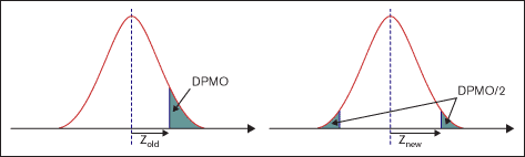
The proposed method of calculating a sigma score sets a measurement boundary where a sigma score of zero represents a 0 percent yield and infinite sigma represents a 100 percent yield. For any specified process yield, the shaded area to the right of center reflects an area equivalent to one-half of the DPMO with the left tail of the curve representing the remaining half. The distance between the inner edges of these areas represents the process sigma.
|
|||||
But accounting for the 1.5 sigma process shift poses a challenge when using this method. The standard way of adjusting for process shift presents a 0 percent yield as either negative 1.5 sigma or positive 1.5 sigma based on whether the baseline data represents a short-term or long-term process performance. In a centered process, if the short-term data provides a 0 percent yield, the long-term performance supports a 0 percent yield, so there is nothing worse than a 0 percent yield. To account for these anomalies, practitioners may apply the scale adapted by Dr. Maurice Berryman, a Six Sigma consultant who is credited with the creation of a scorecard that uses a multiplier to account for long- and short-term process variations. The method uses a factor of 1.3 to convert between these performance values.
For illustration purposes, suppose a process carries a yield of 80 percent. Assume the process is centered, represents long-term variability and includes a 10 percent reject area on each end of the distribution. Using the proposed method of calculating the Z-score, the 10 percent reject area on the right side of the curve provides a Z-score of 1.282 as opposed to 0.842 using the current calculation method. Table 2 shows the values of Z-scores using the current (old) and proposed (new) methods with adjustment for long- and short-term capability. The new method is illustrated in Figure 2.
Table 2 indicates that for the same amount of yield improvement, the change in process sigma value is higher for a process with an initially higher yield when using this method.
| Table 2: Comparison of Process Performance Scores Obtained Using Current and Proposed Methods | |||||
| Current Method | Proposed Method | ||||
| DPMO | Percent Yield | Z-Score Long Term | Z-Score Short Term | Z-Score Long Term | Z-Score Short Term |
| 1,000,000 | 0 | negative infinity | negative infinity | 0 | 0 |
| 999,996.6 | 0.00034 | -4.5 | -3 | 0.0000043 | 0.0000056 |
| 999,000 | 0.1 | -3.09 | -1.59 | 0.0012533 | 0.00163 |
| 990,000 | 1 | -2.326 | -0.826 | 0.012533 | 0.0163 |
| 900,000 | 10 | -1.28155 | 0.218 | 0.12566 | 0.1634 |
| 800,000 | 20 | -0.8416 | 0.6584 | 0.2533 | 0.3293 |
| 700,000 | 30 | -0.5244 | 0.9756 | 0.3853 | 0.5009 |
| 600,000 | 40 | -0.2533 | 1.247 | 0.5244 | 0.6817 |
| 500,000 | 50 | 0 | 1.5 | 0.6745 | 0.8768 |
| 400,000 | 60 | 0.2533 | 1.7533 | 0.8416 | 1.094 |
| 300,000 | 70 | 0.5244 | 2.0244 | 1.0364 | 1.3473 |
| 200,000 | 80 | 0.8416 | 2.3416 | 1.2816 | 1.6661 |
| 100,000 | 90 | 1.2816 | 2.7816 | 1.6449 | 2.1384 |
| 10,000 | 99 | 2.326 | 3.826 | 2.5758 | 3.3485 |
| 1,000 | 99.9 | 3.09 | 4.59 | 3.2905 | 4.2776 |
| 3.4 | 99.99966 | 4.49985 | 5.99985 | 4.64505 | 6.03856 |
| 0 | 100 | positive infinity | positive infinity | positive infinity | positive infinity |
The proposed calculation method redefines the scale from 0 to infinity as well as demonstrates the usefulness of using a multiplier to accommodate for long- and short-term variations. The effect of changing the scale and calculation method also helps address concerns associated with the metric accounting for the relative effort required to improve a process at different levels of initial yield. The method demonstrates that these objectives are aligned with Six Sigma philosophies and provides a more robust and useful performance-reporting process.
About the Author: Dr. Ravindra Kumar ‘Ravi’ Pandey has more than 15 years of experience in the areas of product development, business and operational excellence, Six Sigma strategy and deployment, and business strategy. He has published works about engineering and Six Sigma, holds patents, and is listed in Who’s Who in the World. Dr. Pandey is president of Bipro Inc. He can be reached at [email protected].
Acknowledgement: The author would like to thank Mr. Thomas Rollins of Siemens Power Generation, Orlando, Fla., for his valuable contributions in completion of this article.