This paper looks at some of the methods of estimating standard deviation (which I will usually refer to as ‘sigma’). Additionally, I propose a new formula for estimating sigma for small sample sizes and also present a means to mathematically evaluate these competing estimates of sigma.

The question was posed to me: “I have five samples to test from my population. From that data, how can I estimate capability against our specifications?” Of course, the brutally honest answer is, “Poorly.”

But Black Belts do not survive by being sarcastic, so a better answer might be: “Any estimate of sigma from a small sample will have very large confidence intervals, giving you little knowledge of the actual population.” The question, however, pointed me toward an interesting avenue of exploration into the various ways that we may estimate the sigma in small sample sizes.

Ways of Estimating Sigma

First, let’s review some of the more common methods of estimating sigma (or standard deviation, SD):

A. Using the average difference between an observation and the mean adjusted by sample size (the classic formula for sigma).

B. Using the range of the data divided by a factor, C, where C varies with sample size. Common values of C include 4 and 6, depending on sample size.

SD = Range/C

C. Using the moving range (MR) of time ordered data (where we subgroup on successive data points), divided by a factor. This is the method used in individual moving range control charts.

SD = MR/1.128

D. Using the interquartile range (IQR) of the data divided by a factor (D) where D = 1.35 is the most commonly proposed value.

SD = IQR/D

E. Using the mean of successive differences (MSSD) to estimate variance.¹

F. Using the mean absolute deviation (MAD) , absolute deviation (AD) is an estimate for SD.²

G. Also, you can use the data minimum, maximum, and median to calculate an estimate of variance for small sample sizes.

For the purposes of my study I chose to evaluate all of the methods except for F. I chose methods to study that were easy to calculate (B, C, D), were available in Minitab (A, E) and sparked my interest (G).

Criteria for an Improved Sigma Estimate

A successful search for a better estimate of sigma, when the sample size is N ≤ 10, would meet the following two criteria:

1. The center of the estimates would be equal to the true population sigma.
2. The variation of the estimated sigma would be tighter than the variation observed when using the classic formula for standard deviation.

In other words, if I repeatedly take random samples from a normally distributed population and calculate sigma, then all my samplings of sigma should begin to form a distribution with the average estimate of sigma equaling the true sigma of the data. Improved estimates of sigma will have a tighter distribution of estimates from this repeated sampling than other methods.

(Note: I will be primarily using a visual analysis of dot plots of the distribution of estimates of sigma to evaluate each method of estimating sigma.)

I also calculated the absolute deviation from true sigma (ADTS) using a formula similar to the mean absolute deviation (Method F) in order to numerically gauge each method’s performance against the criteria using the formula:

where Xi is each individual estimate of sigma generated in the simulation and sigma (σ) is the true population standard deviation from which the random normal data was calculated. In this case, N is the number of total estimates in the simulation. This formula sums the absolute value of the difference between each estimate of sigma and the true sigma of the population and divides by the number of estimates. The higher the ADTS factor, the worse the estimation of sigma. (Note: The distribution of standard deviation is a chi-square distribution and is, therefore, not evenly balanced about the mean. This unbalance can be seen in some of the simulations, but was not always clearly observed.)

Method of Evaluation

Minitab’s Random Data calculator was used to create random normal data for testing of the various methods. I decided to study only normally distributed data sets as calculating sigma for the purposes of this article.

I used Minitab to create thousands of random normal data points. These thousands of pieces of data were then sampled using varying sample sizes, from 5 to 50 samples. In most of my explorations that follow, I used 5,000 pieces of random normal data.

Out of the 5,000 random normal data points, I used the following:

• 1,000 five-piece samples
• 500 10-piece samples
• 200 25-piece samples
• 100 50-piece samples

From all these samplings of the random data, I could then calculate the sigma using each of the methods. This gave me a set of data for each method of calculating sigma. A dot plot clearly shows the spread and frequency of each of the estimates of sigma. I could have used other displays of this data such as the classic histogram, but I felt that the dot plot improved the visual clarity of the data.

For example, the dot plot shown below in Figure 1 was created from selecting 1,000 five-piece samples out of 5,000 pieces of random normal data with mean = 0 and sigma = 1. The sigma was calculated for each of these 1,000 five-piece samples using the classic formula (Method A).

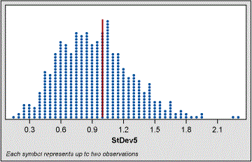
We observe from the dot plot the range of all 1,000 estimates of sigma. As the population was created using a sigma of 1, we can add that line to the dot plot and observe how all of the 1,000 estimates of sigma gathered about the “true” value. In real life we would never know that true value unless we had some previous knowledge from a larger sample. What this shows us is that if we take five random samples from a population where the actual sigma is 1.0, we might get a sigma anywhere from as low as 0.2 to as high as 2.3.

Calculating the ADTS factor for this set of sigma estimations gives us a value of 0.28. Values of ADTS can be compared to each other as long as the estimates of sigma come from the same population (same population mean and sigma).

Evaluation Methods for Estimating Sigma

A randomly generated set of 5,000 normally distributed data points with mean = 0 and SD = 1 was used to evaluate the various candidates for estimating sigma.

Moving Range Evaluation (Method C)

Using the moving range (average MR/1.128) for an estimate of sigma is problematic as it requires that the data is in time order. If we have a small sample size of data and if the order of this data is either unknown or not relevant, then using MR to estimate sigma is not valid.

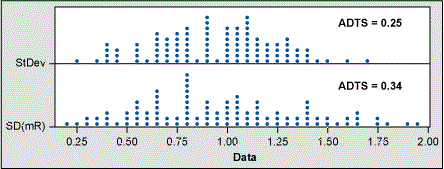
N < 10, the MR is a better estimate of sigma than the classic formula. I performed a test of this using a smaller subset of my normal population dataset and calculated sigma using both the classic formula and the MR. Figure 2 below shows that sigma calculated from MR gives no obvious advantage over the classic formula. The calculated ADTS values support this conclusion.

MSSD Evaluation (Method E)

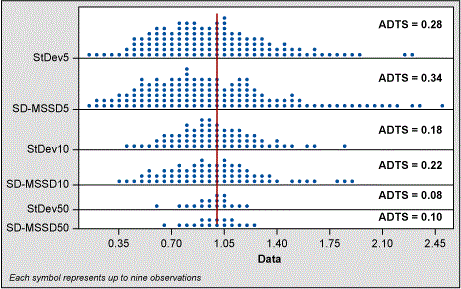
From my 5,000-piece random normal data set, I calculated sigma using the classic formula (Method A) and compared that estimate to the SQRT (MSSD) method. Using Minitab’s Store Descriptive Statistics function along with the calculator function, I compared these two methods for sample sizes of 5, 10 and 50.

As can be seen in the dot plot comparison and ADTS values in Figure 3, the two methods have nearly identical centers and spread. Note that the value of ADTS becomes smaller as the sample size increases. This is as expected since the estimate of sigma improves as sample size increases. Given that the MSSD method provides nothing new over the classic formula, I dropped MSSD from the rest of my evaluations.

The “Hozo” Method (Method G)

In their article, “Estimating the mean and variance from the median, range, and the size of the sample,” mathematicians Stela Pudar Hozo, Benjamin Djulbegovic and Iztok Hozo proposed Method G for estimating variance and, thereby, SD involving sample size, minimum value, maximum value and the median.³

The authors used simulations and “determined that for very small samples (up to 15) the best estimator for the variance is the formula” shown here as Method G.

I tested this formula using my 5,000-piece population of random normal data and compared to the classic sigma formula as shown in Figures 4 and 5.

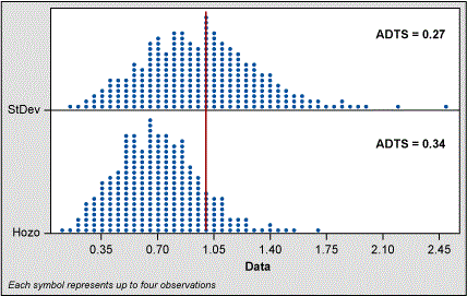
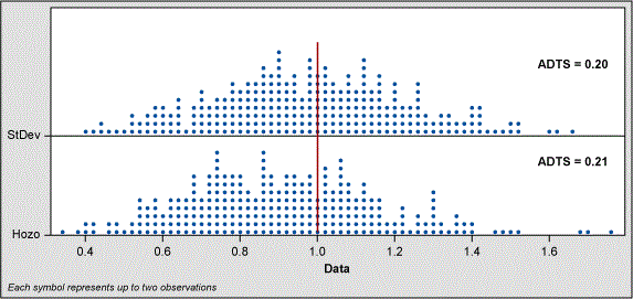
When the sample size is five, the Hozo method shifts the range of estimates to the left. Even though the spread of estimates is better for the Hozo method, the ADTS values show the classic standard deviation formula is slightly better. At the sample size of 10, the shift is not as great and the ADTS values indicate little difference between the classic sigma and Hozo methods.

However, in fairness to Hozo et al, their study parameters were different from mine. Instead of a mean of 0 and sigma of 1 (which I used to create normal data), they “drew 200 random samples of sizes ranging from 8 to 100 from a normal distribution with a population mean [of] 50 and sigma [of] 17.” This is a large sigma when compared to the mean (17/50). I am not sure that is practical in engineering.

Therefore, I created 5,000 random normal data points using mean = 50 and SD = 17 to see how the Hozo method compared to the sigma formula for a sample size of five and 10. This simulation still shows that with N = 5 the estimate of sigma is shifted away from the actual population sigma of 17. For N = 10 the shift is less but still present. The ADTS values bear out this conclusion.

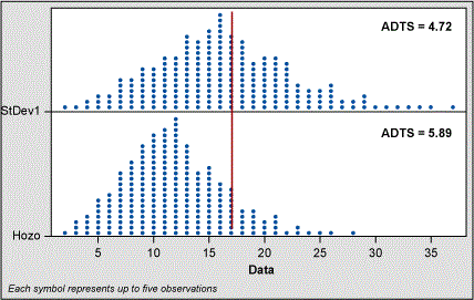
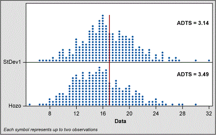
In their study, Hozo et al found that “when the sample size increases, range/4 is the best estimator for the sigma until the sample sizes reach about 70. For large samples (size more than 70)[,] range/6 is actually the best estimator for the sigma (and variance).”

Range/C (Method B) and IQR/D (Method D) Evaluation
While all the other formulae are definitive in their variables, the range and IQR methods require some way to decide what to use for the values of C and D.

SD = Range/C

SD = IQR/D

From Hozo et al I found that commonly used values for C are 4 and 6, and that the most commonly used value for D is 1.35.

I decided to test these values against alternate values of C and D in the hopes of finding an improved range or IQR formula for small sample sizes (e.g., <10). After preliminary modeling using a wide selection of values for C and D, I settled on testing the following factors:

• Range (R)/C where C = 2.5
• IQR/D where D = 1.35 and 1.55

Once I determined the values of C and D to be evaluated, I used the 5,000 pieces of random normal data to calculate the spread of estimates of sigma using values of C and D as defined above and compared them to the classically calculated formula for sigma along with their ADTS factor.

In the dot plots that follow I left out the plots of the classic sigma formula as I am focusing on the centering and spread of the various estimates using R/C and IQR/D.

The code of labeling is as follows:

• Range 5/2.5 means range data from the sample size = 5 group divided by 2.5
• Range 10/2.5 means range data from the sample size = 10 group divided by 2.5
• IQR 5/1.35 means IQR data from the sample size = 5 group divided by 1.35
• And so on

Range Evaluation

Figure 8 shows that R/4 is greatly left-shifted when N < 10 and that R/2.5 is centered – although the spread of the R/2.5 data is large. At values of N > 10, using R/4 centers around the true sigma much better than R/2.5.

Plotting all the ADTS factors by sample size and sigma calculated by R/C and classic standard deviation shows how R/2.5 and R/4 change with sample size (see Figure 9). We also can see how these estimates of sigma compare to the classic standard deviation formula.

IQR Evaluation
In Figure 10, the IQR/D estimates show that when the sample size is 5 or 10, then IQR/1.55 is more centered and has less spread of estimates than when compared to IQR/1.35. With sample sizes greater than 10, however, this pattern shifts and IQR/1.35 slightly improves.

As with the range data, I plotted the ASTS values for each IQR/D method and compared them to the classic formula for standard deviation (Figure 11).

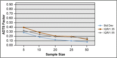
A summary chart of these two methods is shown in Figure 12. This chart shows that all methods are almost equal when N = 5. When N = 10, the IQR/1.55 is better than R/2.5 but not as good as the classic formula for standard deviation.

Taking a Final Look

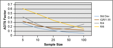
Given that the best estimates for sigma appear to be IQR/1.55, R/4 or R/6 (depending on sample size), I created a new set of 5,000 pieces of random normal data and re-ran all of the calculations of ADTS for each combination.

The graph in Figure 13 is interesting in that it shows how IQR/1.55 is actually pretty robust over sample size. The IQR/1.55 method would be a good choice if picking a method for estimating sigma (that was not the classic formula).

The IQR/1.55 method has another advantage. Both the R/C method and the classic sigma method are prone to outliers, especially with small sample sizes. The IQR/1.55 method is not affected by an extreme outlier in a small sample of data.

For example, let’s look at a set of seven data points to see how an outlier affects our estimates of sigma. Below are two seven-piece random and normal samples of data from a population with a known sigma of 1.0. The first set of data does not have an outlier; the second set of data does have an outlier (2.0) as confirmed by Grubb’s test for outliers.

Table 1: Sample Data
Data 1	Data 1_1
0.229762	0.22976
0.370426	0.37043
0.402137	0.40214
0.589118	0.58912
0.776588	0.77659
0.845852	0.84585
0.969874	2.00000

From this data we can calculate the following estimates of sigma and see how the IQR method is robust to an outlier. The classic method and the R/2.5 method change significantly with the presence of an outlier.

Table 2: Comparing IQR and R to Classic Sigma
	Classic Sigma	IQR/1.55	Range/2.5
No Outlier	0.76	0.307	0.296
With Outlier	0.596	0.307	0.708

For ease of calculations, if you are given a choice, a sample size of N = 7 allows the IQR to be easily solved. For N = 7, the third quartile is the sixth data point in ordered data, and the first quartile is the second data point in the ordered data. When N = 11, then the third quartile is the ninth point and the first quartile is the third point.

Conclusion

A successful search for a better estimate of sigma centers the estimates about the true population sigma and has a tighter spread of estimates than given by the classic formula for standard deviation.

In this study, we examined several candidate formulae for sigma when N ≤ 10. We also hypothesized two new formulae (R/C, where C = 2.5 and IQR/D where D = 1.55).

Other methods of estimating sigma (MSSD, Hozo and MR) do not appear to offer any advantages over the classic formula for sigma. The Hozo method also seems to shift the center of the estimates of sigma to the left of the “true” sigma.

Estimates of sigma using IQR/1.55 appear to be good when the population data is normal – regardless of sample size. Although the classic formula appears to give lower ADTS scores for every sample size.

It is recommended that when the sample size is small, that a test for outliers (e.g., Grubb’s test) be performed. If an outlier exists and if the reason for the outlier cannot be determined, then the IQR/1.55 method is recommended.

The decision by an investigator to use the IQR/1.55 method, Range/C method or the classic standard deviation formula is situational. But it may be argued from this data that the classic formula of standard deviation is the best estimator of sigma – regardless of sample size.

References

1. Estimate process variation with individuals data, Minitab support topics, Minitab.com, Accessed July 9, 2017.
2. Sigma Calculator, NCSS Statistical Software Documentation, https://ncss-wpengine.netdna-ssl.com/wp-content/theme/ncss/pdf/Procedures/NCSS/Standard_Deviation_Calculator.pdf. Accessed July 9, 2017.
3. Hozo, PS, Djulbegovic B, Hozo I. “Estimating the mean and variance from the median, range, and the size of a sample,” BMC Medical Research Methodology. 2005. DOI: 10.1186/1471-2288-5-13.