Statistical process control (SPC) is the application of statistical methods to identify and control the special cause of variation in a process. Control charts, in theory, are used in product and process development to analyze processes. When a process is shown to be in control in both an average and range chart the process can be released for use in production. In practice, however, SPC is often introduced into a production environment where not all processes are in control and fully capable. This article will discuss how best to introduce SPC into such a production environment.

The Three Loops of SPC Implementation

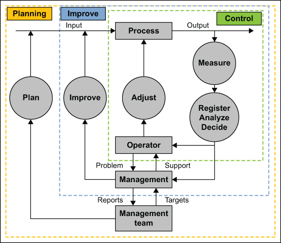
When implementing SPC, activities and responsibilities should be clearly established. In the first loop (control loop, see Figure 1) of SPC, an operator will look at subgroups to address any items that are out of control in the process. When the operator is not able to handle the out-of-control variables in the first loop – or if preventive action is required – the second level should be activated (improve loop). At this stage, production management or engineering personnel can take appropriate actions to avoid recurrence of the problem.

In modern production systems there is not much overcapacity of operators and engineers; the time to work on action plans and improvement activities resulting from out-of-control variables is limited. Clear priorities need to be set by management so that operators, production management and engineers will address the correct problems. This is the third (and final) SPC loop – planning.

Out-of-control Variables

During the implementation of SPC, organizations may have problems managing the amount of items that are out of control in the early stages. The usual reasons for the large number of out-of-control factors include the following:

• Processes are, simply, out of control. In the early stages of an SPC implementation, control charts typically show a large percentage of subgroups are out of control. Examples of out-of-control variables are incorrect measurements and overadjustment of the process by operators.
• When SPC software is used in the SPC implementation, the number of control charts can quickly proliferate. Control limits are calculated automatically and, therefore, every disturbance in the process will lead to an out-of-control signal.
• Characteristics being monitored are often not classified, so all control charts get the same priority. But some charts are extremely important and other charts are used only as help for calculations and are of no real importance. Significance of factors, in order of priority, would come from a failure mode and effects analysis (FMEA).
• In many production environments, the process average is unstable. Reasons for this may include tool wear, setup differences, differences in raw material and machine warm-up times. All of these situations will show out-of-control points on the average (e.g., x-bar) control chart, but for some of these situations, it is not possible to bring the process average into control. For example, it may not be financially feasible. The instability of the process average will be visible with a large difference between C_p and P_p (e.g., P_p/C_p > 1.25).

But what is more important in terms of this reason is that the out-of-control variables on the control chart monitoring the process average will place the emphasis on the wrong chart. The more important control chart is the one monitoring process dispersion (commonly the range or sigma chart) and, in general, this chart should be in control first before attention is given to the average chart.

How to Reduce the Number of Out-of-control Variables

Too many out-of-control points is one of the most common reasons why SPC implementations fail. If there are 30 out-of-control points in a shift and there is only time to address three or four points, then it seems futile to make the effort as progress can never be made. With such dismal prospects for addressing all the problems, operators essentially throw their hands up in defeat. There should never be more out-of-control points than can be addressed.

There are two ways to address the problem of too many out-of-control factors at the early stages of an SPC implementation:

1. Reduce the amount of control charts and only use charts for a few critical quality characteristics.
2. Use control charts for all quality characteristics but widen the control limits of the average chart for non-critical quality characteristics.

The advantage of the first option is that SPC will be used as it is intended to address critical variables. The disadvantage of this option is that severe quality problems can appear on quality characteristics that are not being monitored, in which case limited data would be available for further analysis of the process and for reporting to customers and management.

The advantage of the second option is that all quality data is monitored and can be used for analysis and reporting. The disadvantage of this option is that more effort and knowledge is required to manage the control charts and the calculation of the control limits.

The next section describes an approach to managing control charts during SPC implementation when dealing with the second option.

Calculating Control Limits

At the start of an SPC implementation all efforts must be aimed at controlling the variation of the dispersion (via a range or sigma control chart). When the dispersion of the process is out of control, the average of the process is likely also out of control. This is because there is a relation between the variation in the dispersion and the variation of the average as shown in this equation:

 

 

Problems on the dispersion chart should be addressed first. When control limits on the average chart are calculated in the standard way (three sigma from the average), out-of-control variables on the dispersion chart will also lead to out-of-control factors on the average chart. These out-of-control factors on the average chart are not an indication of changes in the process average, however, but are a logical result of changes in the dispersion. When operators without adequate knowledge of SPC see out-of-control variables on both average and dispersion charts they will likely start working on the “problem” on the average chart because such problems are easier to address – just adjust the process.

The way to avoid this issue is to begin charting without putting the limits of the average chart at three sigma. There are three options:

1. Do not use control limits for the average – only show the target. This is sometimes called a run chart.
2. Fix the limits at a level which will rarely lead to out-of-control variables.
3. When the process average is unstable use modified control limits to minimize the actions, but make sure that process averages that are abnormal are signaled.

When the C_p value is high enough, the third method is preferred because the limits are still calculated based on the process variation. This method still gives an early warning when a disturbance of the process average will lead to defective products.

How to Calculate Modified Control Limits

When the process average fluctuates, a certain amount of fluctuation can be allowed before starting to look for the cause – as long as a required (as determined by the customer or industry) C_pk value is achieved. The control limits may be set at a level such that the C_pk is higher than a required value. In other words, the distance between upper specified limit (USL) and the process average should be higher than:

 

where

 

 

is the estimated standard deviation of the population

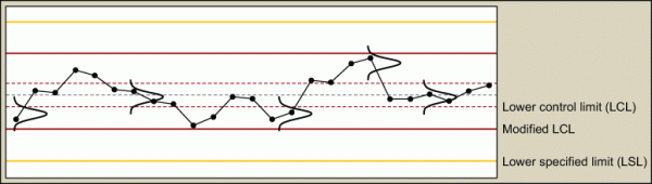
In Figure 2 the dotted red lines are the control limits. The solid red lines are the modified control limits based on a required C_pk value of 1.67 (used in the automotive industry). The yellow lines reflect the upper and lower specification limits although normally these are not shown.

The modified control limits can be calculated as follows. The process average is allowed to shift to a level where the distance between the USL and the process average is

 

 

The distance between the average and the control limit is

 

 

This means that the distance  between the USL and the modified upper control limit is as follows:

 

 

or

 

 

The requirement for using this formula is that the C_p value of the process is higher than the required C_pk. If that is not the case, then the modified control limits will be too close to the process average and result in false alarms.

Using Modified Control Limits

Modified control limits are not recommended for every situation. If it is desirable to find special causes of variation, calculate the control limits in the standard way. Use modified control limits as a method to distinguish between priorities among the different process characteristics being monitored.