
Central tendency is just one measure of a set of data. In this article, we will present the different ways of calculating central tendency, the pluses and minuses of each, and the importance of considering more than just central tendency when describing a set of data.
Overview: What is central tendency?
All processes generate data, whether it be continuous or discrete in nature. All data will form a pattern or distribution. Some common distributions are; normal, binomial, and poisson. All these distributions can be described in terms of three characteristics; central tendency, variation, and shape. Let’s learn more about central tendency.
Central tendency can be defined as the value around which the other data points tend to gather. Regardless of the type of distribution, they all have a measure of central tendency, although they may be calculated in different ways. The mean (often referred to as the average) of a data set is the most frequent measure of central tendency. Sometimes you will see the average referred to as location.
The formula for calculating it is:
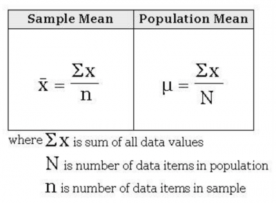
Notice that the notation for the mean is slightly different if you are referring to the mean of a population (mu) or a sample (Xbar). The other two common measures of central tendency are the median and the mode. Why do we need two other measures of central tendency?
The mean is the calculated center of the data. One of the limitations of the mean is it can be skewed by an outlier. In other words, an unusually high or low value in the data will cause the mean to shift away from the physical center to something higher or lower, resulting in a skewed distribution.
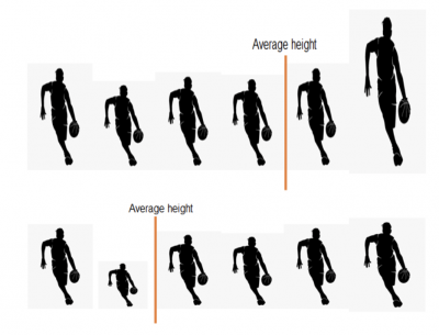
Let’s assume we have six basketball players of approximately the same height. You can see the average height of those players would be somewhere near the middle of their individual heights.

But, what would happen if the team recruited a really tall superstar? The average height would shift to the right. Likewise, if they recruited a really short player, the average would skew to the left.
We may conclude the average alone may not always be an accurate measure of central tendency.
The second common measure of central tendency is the median. It is defined as the physical center of the data after the data has been sorted either high to low or low to high. Half of the values will be above the median, and half below.
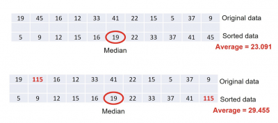
The median is not influenced by an outlier. If you have an odd number of data points, the median will be the number in the middle, once sorted. If you have an even number of points, the median will be the average of the two values in the middle. In the example below, notice how the mean changes with the addition of a large outlier but not the median.
It is recommended to look at both the mean and median together. If both are similar, you can conclude there are no extreme outliers, and your data should not be skewed. If your mean and median appear to be different, you should examine your data for outliers.
The third measure of central tendency is the mode. It is defined as the most frequently occurring number in your data set.
The mode becomes interesting if your data has multiple modes. This may mean you have combined two sets of diverse data and should consider separating and analyzing them separately.
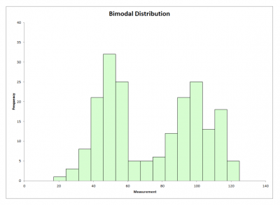
For example, if you look at the payment times for your accounts receivables below, you will see a bimodal, or two-mode distribution. You should examine the fast payers and slow payers separately to understand why one group pays quickly and the other doesn’t.
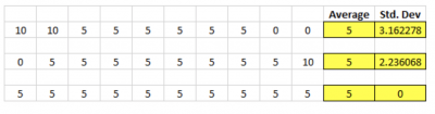
Relying solely on central tendency to understand your process data can be deceiving without a measure of variation. Looking at the three examples below, you will see they all have the same average but are different data sets if we look at the standard deviation.
2 benefits and 2 drawbacks of central tendency
The central tendency of a set of data is a fundamental concept in statistics and mathematics. But, care must be taken in drawing too many conclusions about your data just based on central tendency.
1. Central tendency is simple to calculate
The calculations for mean, median, and mode are simple to do and don’t even require a calculator.
2. Provides an indication of the center of a data set
The mean is the calculated center, while the median is the physical center.
3. Can be influenced by extreme values
The average can be skewed by an outlier in the data, giving you a false impression of where the center really is.
4. Does not address variation
Without a measure of variation in the data, central tendency only gives you a portion of the information about your data and your process.
Why is central tendency important to understand?
Understanding the central tendency of your data gives you a sense of where the total set of data will gather.
Mean vs median
Use both the mean and median to tell you about your data. Since the mean can be influenced by outliers, compare it to the median. If both are close, then outliers may not be a problem.
Importance of the mode
If your data contains more than one mode, it might be an indication you have combined data from different conditions and should be analyzed separately.
Central tendency without a measure of variation
Without a measure of variation, your central tendency only gives you a partial understanding of your data.
Concept applies to discrete as well as continuous or variable data
The concept of central tendency applies to every type of data distribution even though the calculations will be different.
An industry example of central tendency
The VP of logistics approached the company’s Master Black Belt (MBB) and asked her to get involved in an analysis of on-time delivery to the company’s customers. The metric they were using was the number of days from the order being ready to ship until it arrived at the customer’s loading docks.
The VP was told the average delivery time was 7.58 days. In his opinion, this was too long and something needed to be done.
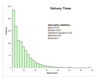
The MBB took delivery data for the last six months and entered it into her statistical software program. She confirmed the average delivery time for the past six months was actually 8.46 days. She noticed the median was 6.09, which was less than the average. In looking at the histogram, she saw the distribution of delivery times was heavily skewed because of the number of very late deliveries.
While six days was still long, the VP was relieved to see it wasn’t as high as the average had indicated. The MBB put a team together to try and reduce delivery delays and the reasons for the very late deliveries.
3 best practices when thinking about central tendency
Despite the simple calculations related to central tendency, there are a few tips to keep in mind to gain a complete understanding of your data and, thus, your process.
1. Always look at both the mean and median
Outliers may cause your mean to distort the true central tendency of your data. Always compare the mean and median of your data to see if there was any influence from outliers.
2. Describe your central tendency along with a measure of variation
Use either a range, standard deviation, or variance of your data to accompany your measures of central tendency.
3. Don’t forget to sort the data if calculating the median
The median is the data point in the middle, but only if the data has been sorted from high to low or low to high.
Frequently Asked Questions (FAQ) about central tendency
What are the most common measures of central tendency?
The mean, median, and mode.
What is the advantage of using the median?
The median provides a good measure of the central tendency and is not influenced by the presence of outliers in the data.
Is there ever a case where the mean, median, and mode are the same?
Yes. In a normal distribution, the values of the mean, median, and mode will be the same, and the shape will be symmetrical.
Central tendency — useful or not?
The use of central tendency to describe your data is one important descriptor. It describes the value data points will tend to gather around. The most common measures of central tendency for continuous data are the mean, median, and mode. The mean is the calculated center. The median is the physical center, and the mode is the most frequently occurring value.
The mean can be influenced by outliers, so it is recommended you compare the mean and median to see if your mean has been skewed. Finally, your central tendency only provides a portion of the information you need to understand your data. Always accompany your description of central tendency with a measure of variation (a.k.a., spread or dispersion).