
Many statistical tools make an assumption your data distribution is normal. That will not necessarily be the case. If you want to analyze your data and it is not normally distributed, you have a few options. One of those options is to transform the data using either a Box Cox or Johnson transformation. This story describes how a company came to the conclusion they needed to do a transformation and what happened when they tried using the Box Cox and Johnson transformations.
The company’s Master Black Belt (MBB) was having difficulty analyzing some of the company’s process data.
The company’s newly hired MBB, Steve, started to learn about the company’s processes by reviewing their data collection procedures, data structure and then analyzing some of their key KPIs. The first analytical tool he tried was a 2-sample t test to see if the recent changes on the production line statistically reduced the changeover time on their equipment.
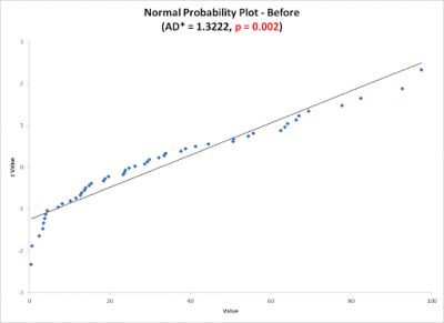
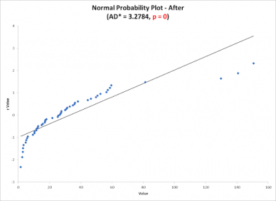
One of the underlying assumptions for using the 2-sample t test is that both groups of data are normally distributed. Unfortunately, since he was measuring time, the data is not expected to be normal since time has a natural lower boundary of zero and an infinite upper boundary. Shown below is what the normal probability plot looked like for his two sets of before and after data. Note the low p-values indicating the data is different than normal.
At this point, Steve had a few options to determine whether the process changes were significant. First, he went back and looked at the data and how it was collected to see if the problem was due to some data collection error. He also investigated whether an MSA was done to determine if the data could be trusted. Neither of those explained the non normality of the data. Steve concluded the nature of the process would typically produce non normal data since the metric was time.
The next decision was whether to use a nonparametric test for comparing the two data sets. A nonparametric test does not have an assumption of a specific distribution so the issue of normality is not relevant. The common nonparametric test for comparing two data sets is the Mann-Whitney test. But, nonparametric tests compare the medians of two populations while the parametric test compares the means of two populations. In many cases, parametric tests have more power. If a difference actually exists, a parametric test is more likely to detect it. Since Steve was interested in the means, he discarded the idea of using a nonparametric test.
That left Steve with one of two remaining options. He could either do a transformation of the data using a Box Cox transformation and then use a 2-sample t test or he could use a Johnson transformation and again use a 2-sample t test.
Steve decided to use a data transformation so he could analyze the company data.
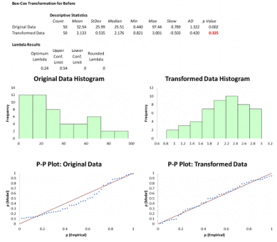
The Box Cox transformation is named after statisticians George Box and Sir David Cox who developed the technique in 1964. At the core of the Box Cox transformation is an exponent, lambda (λ), which varies from -5 to 5. All values of λ are considered and the optimal value for your data is selected. The optimal value is the one which results in the best approximation of a normal distribution by finding the value of lambda which minimizes the standard deviation between the default values of -5 and 5.
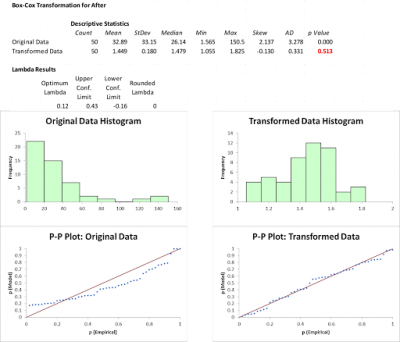
The charts below show the Box Cox transformations for the Before and After data. Note the p-value is greater than .05 which tells you the transformed data is not different than normal. You can also see the shape of the histograms and the normal probability plots.
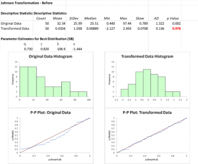
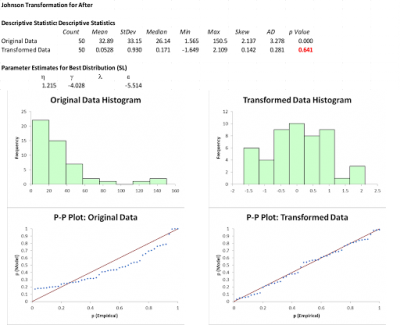
Although Steve was happy the Box Cox successfully transformed his data, he wondered if the Johnson transformation would provide better results. While the calculations for Johnson are more complex than the Box Cox, Steve didn’t worry since all the number crunching was being done by his statistical software. Here is what the Johnson results looked like. Notice how much larger the p-values are therefore demonstrating the power of the Johnson transformation versus the Box Cox. Also, the histograms and probability plots are more representative of a normal distribution.
Now that the transformed data was approximately normal, Steve could do his 2-sample t test to see if there was a statistically significant improvement in changeover time. Steve had similar issues with some process capability analysis he wanted to do so he used the data transformations rather than the more complex techniques of identifying what the actual distributions were and then doing a non normal capability analysis.
While doing the transformation calculations was easy thanks to the use of software, explaining that transformations were not magic or a tricky way to change the data was more of a challenge.
It took Steve literally a minute to run the actual calculations using his computer and statistical software. The bigger challenge was getting lay people to understand that transformations are not distorting or changing the data but presenting it in a different format. The underlying values of the data are retained but are represented in a different format.
Steve used the analogy of taking a trip to Europe. For your trip, you took $100 USD with you. Unfortunately USD was not easily accepted so you had to transform your dollars to Euros. To do that, the exchange booth at the airport did a mathematical transformation of your dollars to an equivalent amount of Euros. The resulting amount of Euros had the same underlying worth as your dollars but were in a different form of paper money and coins. In this transformed unit, you can now do what you need to do. When you are ready to return to the US, you will stop by the same exchange booth and they will do a back transformation where they will transform the Euros back to dollars.
There is one major caution associated with transformations. The transformed data is not in the same units as the original data. If Steve’s original data was in minutes, his transformed data might be represented as Y^lambda where Y is the original data point taken to the power of lambda. This can be confusing, so be careful about tossing around the transformed data. It might not make sense to someone not well versed in transformations.
Where applicable, Steve’s use of data transformations enhanced his analysis.
While Steve’s ability to do his analysis on the turnaround time was enhanced by his use of data transformations, it should be the last thing you try, not the first. Don’t rush to transform data if it isn’t normal. Where appropriate, you can use non parametric statistical tools. In many cases, the statistical tool will be robust or forgiving with respect to normality. One of the big controversies is whether to transform your data for use in a control chart. Except for a possible few exceptions, the control chart is robust to normality. Since a control chart is meant to be displayed for monitoring your process, it would be very confusing to the reader if the values on the control chart were some transformed number which would make no sense or relate back to the metric you are measuring.
3 Best Practices If You Decide You Want to Transform Your Data
Here are a few hints of what to do if you decide your data needs to be transformed to be useful.
1. Make sure your data is trustworthy
Be sure to do an MSA on your measurement system to be confident your data represents reality.
2. Understand the nature of your process data and what analysis you want to do
Some data may not be normal by virtue of your natural process performance. In that case, transformation may be appropriate. You must understand what statistical tool you want to use and the underlying assumptions which must be met to use it. You must also decide whether the simplicity of the Box Cox transformation is adequate for what you want to do or the more powerful Johnson transformation is needed.
3. Be careful about sharing transformed data
Since your transformed data is no longer in the same units as your original data, be careful about displaying and sharing your transformed data. You don’t want to create unneeded confusion in people trying to make use of your analytical work.
Transforming the data worked for this company and it may work for you as well.
While the normal distribution is a good representation of many processes and real life situations, it does not necessarily hold for all data. Transforming the data should only be used as a last resort if the statistical analysis you want to perform has normality as an underlying assumption.
Data transformation is not magic nor an attempt to obfuscate the original data. Its purpose is to reformat the data to make it more useful in certain statistical applications. Since the transformed data is in different units you need to be careful about people trying to interpret and make decisions using the transformed values they see. If you are a data analyst you might want to transform your data as needed, do your analysis, back transform the data and then present the results to your audience.