Determining the distribution of your data is often the first step in analyzing your data. One distribution in particular, the normal distribution, is an underlying assumption for many of the  statistical tools you might use to analyze your data. Failing that assumption might require you to use a different statistical tool or approach. 

This article will explore what normality is and how the value of A-square can be used to confirm whether you meet your normality assumption. We will also explain the benefits of the A-square calculation as the output of the Anderson Darling Normality Test (AD) and offer a few tips for understanding when and how to use A-square.  

Overview: What is A-square? 

A-square is the test statistic for the Anderson-Darling test. It is used to test whether a data sample comes from a specific distribution. It can be used to test whether your data meets the assumption of normality.

Normality refers to a specific statistical distribution called a normal distribution. It is described as a symmetrical continuous distribution defined by the mean and standard deviation. The mean, median, and mode of the data are the same for a normal distribution.

The normal distribution is a hypothetical distribution defined by:

What you are really confirming with the AD test and A-square is whether the distribution of your data is close enough to normal you can state you fulfilled the normality assumption to use your selected statistical tool for analysis. 

The AD test is really a hypothesis test. The null hypothesis (Ho) is that your data is not statistically different from a normal distribution. Your alternate or alternative hypothesis (Ha) is that your data is different from a normal distribution. The decision whether to reject or not reject the null is based on your p-value. 

The formula for the test statistic A-square is:

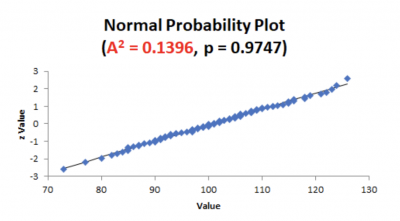
Here is an example of a probability plot that provides the results for A-square. 

Note that the value of A-square is 0.1396 and the p-value is 0.9747. The 0.1396 was calculated from the A-square formula shown above. Given a p-value of 0.9747, you would not reject the null that your data is not different from normal. 

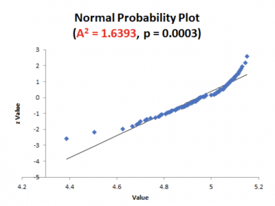
Let’s look at another example.

This time, notice that the p-value is 0.0003 based on the A-square value of 1.6393. You would now reject the null hypothesis and conclude your data is different from normal. 

As the value of A-square increases, the value of p will decrease. In other words, small values of A-square will indicate your data is statistically the same as a normal distribution. Large values indicate your data is statistically different from normal.

3 benefits of A-square 

Should you or shouldn’t you reject the null hypothesis concerning the normality of your data? A-square provides the answer to that question. 

1. Provides guidance for your decision 

A-square is used to calculate your p-value. This will provide guidance on whether to reject or not reject your null hypothesis. 

2. Can be simple 

Fortunately, you will not have to do the complex hand calculations to determine A-square. Today, computer software is available to provide you a graphical picture of the data along with the A-square and p values. This information will give you confirmation about the distribution of your data. 

3. Confirmation of the shape of your data 

Remember, the normal distribution is a hypothetical distribution. You can’t prove that your data is normal but rather if your data is not normal. The AD test can be used to test any distribution, not just the normal.

Why is A-square important to understand? 

In addition to an underlying assumption of normality for certain statistical tools there are a number of other types of distribution for other tools. For example, Binary logistic regression has an assumption of the binomial distribution. Other statistical tests might have an assumption of F or Chi-Square distributions. 

Interpretation of p-value 

The p-value, calculated using A-square, will tell you whether you can reject your null hypothesis or not. It’s important to know the relevance so the next action you take is appropriate.  

The impact of sample size 

The value of A-square will vary as a function of the size of your sample. As your sample size gets large, the sensitivity of your AD test may tell you the data is non normal when, in reality, it is. Don’t rely on graphs except as a directional indicator. Rely on the A-square and p-value to tell you how to react to your null hypothesis. 

The relationship between A-square and your hypothesis test

The AD test is a form of hypothesis testing. The AD statistic, also denoted as A-square, provides you the information on what decision to make about your null hypothesis.

An industry example of A-square 

A sales manager wanted to confirm whether the recent revision of the incentive plan had an impact on sales for his four sales offices. He had daily sales data for 60 days before the revision and 30 days after the revision. He wanted to compare the average sales for his four divisions.

He decided to consult with his Lean Six Sigma Black Belt, Barbara, on how to analyze the data.

Barbara advised that, since the manager was interested in comparing four sets of continuous data, the appropriate test was ANOVA. An underlying assumption is that the sample data for the four sales offices will be normally distributed. 

Upon checking the normality of the data with the Anderson-Darling test, Barbara found the data not to be normally distributed. Therefore, she was not comfortable just doing the ANOVA test even though she knew her sample size was pretty large and ANOVA is somewhat robust to the assumption of normality.

She decided to use the nonparametric Mood’s Median test, which does not have an assumption of normality. In the end, the p-value computed from the AD A-square calculation and the p-value of the Mood’s Median test led to the same conclusion. The results showed that the revised incentive plan was statistically effective for two of the four offices. The sales manager went to work trying to understand why it didn’t work in the other two.

3 best practices when thinking about A-square 

Here are a few tips to help you gain insight into using A-square to confirm the distribution of your data. 

1. Use graphics and charts 

While graphics are best used as a directional indicator, sometimes a simple plot of the data such as a histogram or probability plot will provide useful insight into what your data distribution might be. You should use statistics to confirm any visual conclusions. 

2. Choose your sampling technique 

Your sampling technique and sample size will impact your final calculations and decisions. Random sampling is used to reduce the amount of sampling bias you might have.

3. Have a Plan B

In the event your data is not normally distributed, don’t despair. In most cases, there are alternative statistical tools you can use to help you get the answer to your statistical questions. 

Frequently Asked Questions (FAQ) about A-square

1. What is the difference between the Anderson Darling Test and A-squared? 

The actual test for identifying the type of distribution was named after Theodore Anderson and Donald Darling. A-square is the test statistic or formula used to calculate the Anderson Darling value. This value is then used to compute the p-value, which provides the necessary information on whether to reject or not reject the null hypothesis associated with the Anderson Darling Test. 

2. Can the value of A-square be used for distributions other than normal? 

Yes, while the AD test and A-square are commonly used for testing the assumption of normality, the AD test can be used for any distribution. 

3. Are there other tests for normality besides AD? 

Yes, there are a number of other tests. One of the more popular tests is the Kolmogorov-Smirnov (K-S) test. Other commonly used tests are the Ryan-Joiner and Shapiro-Wilk tests. Each of these tests has its own test statistic that’s used to compute p-value.

Final comments on A-square 

Many statistical tools have an underlying assumption that your data needs to be approximately normally distributed. If it’s not, you must seek a different tool to answer your statistical question. The good news is many of the tests requiring normality are robust to that assumption. In other words, your eventual answer won’t be too different if you violate the assumption of normality.

The AD test starts with the null hypothesis that your data is not statistically different from normal, with the alternate hypothesis being it is different from normal. The A-square value of the test statistic and subsequent p-value will suggest you can either reject the null, or must fail to reject the null.