Key Points

• The AD test is intended to test for normality in a given sample set.
• Using the test allows you to see if your sample fits within a normal distribution.
• The Anderson-Darling Test is a hypothesis test, that allows users to test for a null hypothesis.

What exactly is an Anderson-Darling test? Testing for normality is often the first step in analyzing your data. Many statistical tools you might use have normality as an underlying assumption. If you fail that assumption, you may need to use a different statistical tool or approach.

This article will explore what the normality of the data means and how the AD test can be used to confirm whether your data will satisfy the assumption of normality. We will also explain the benefits of the AD test and offer a few best practices for understanding when and how to use the AD test. 

Overview: What Is the Anderson-Darling Normality Test (AD test)? 

The Anderson-Darling test is used to test if a sample of data comes from a population with a specific distribution. Its most common use is for testing whether your data comes from a normal distribution. 

But, what does that mean? 

Normality refers to a specific statistical distribution called a normal distribution, or sometimes the Gaussian distribution, or a bell-shaped curve. The normal distribution is a symmetrical continuous distribution defined by the mean and standard deviation of the data.

The normal distribution is theoretical. What you are testing with the AD test is not whether your data is exactly consistent with a normal distribution, but whether your data is close enough to normal that you can use your statistical tool without concern. 

In some cases, a statistical tool may be robust to the normality assumption, which means the statistical tool is not overly sensitive to some level of violation of the normality assumption. The normal distribution is popular because it describes many real-life situations, such as the distribution of people’s heights, weights, and income.

The AD test is a hypothesis test. The null hypothesis (Ho) is that your data is not different from normal. Your alternate or alternative hypothesis (Ha) is that your data is different from normal. You will make your decision about whether to reject or not reject the null based on your p-value. 

The test statistic for the AD test is:

Yes, I know it looks really scary, but don’t worry. All the computations can be done by statistical software on your computer. The output you get will include a p-value. 

Assuming you selected your alpha risk to be 0.05, you will reject the null if the p-value is less than 0.05. That allows you to claim that your data is statistically different from a normal distribution. On the other hand, if your p-value is higher than 0.05, you can state that your data is not statistically different from a normal distribution.

Examples of an Anderson-Darling Test

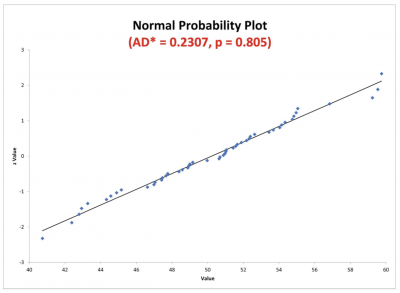
Here is an example of a probability plot that provides the results for the AD test. 

Note that the value of the AD statistic is 0.2307 and the p-value is 0.805. The 0.2307 was calculated from the AD formula above. With a p-value of 0.805, you would fail to reject the null and conclude that your data is not different than normal. This would satisfy any assumption of normality you might need for a statistical test. 

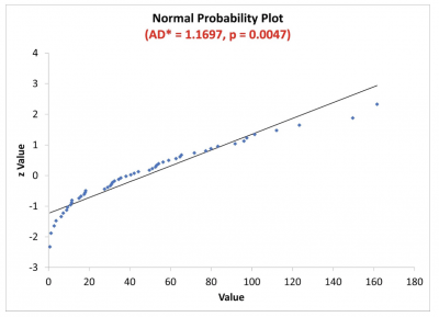
Let’s look at another example.

This time, notice that the p-value is 0.0047 based on the AD statistic of 1.1697. In this case, you would reject the null hypothesis and say that your data is different than normal. 

Benefits of the Anderson-Darling Normality Test (AD test) 

Knowing the underlying distribution of your data is important so you can apply the most appropriate statistical tools for your analysis. 

Confirm Your Data Distribution

The AD test will help you determine if your data is not normal rather than tell you whether it is normal. Since the normal distribution is a hypothetical distribution, you can’t prove that the data is normal. The AD test will tell you if it is not normal or if it is not different from normal, but it cannot tell you if the data is normal.

Helps Guide Your Decision

The p-value, which is based on the value of the AD statistic, will provide you guidance on whether to reject or not reject your null hypothesis.   

Can Be Simple 

In many cases, the computer software you use will provide you with a graphical representation of the data along with the AD value and p-value. This will give you some visual and logical confirmation about your data. 

Why Is the AD Test Important to Understand?

Different statistical tools for analysis have different assumptions regarding the underlying distribution of the data that you are analyzing. 

For example, the t-test has an assumption that the data is normally distributed. Linear regression assumes that the underlying distribution of the residuals is normal. Binary logistic regression has an assumption of the binomial distribution. Others might have an assumption of the F or Chi-Square distributions. 

You need to understand what these assumptions are regarding your data. 

What Is Your Hypothesis Test?

Since the AD test is a form of hypothesis testing, you want to correctly state your null and alternative or alternate hypotheses. In the case of the AD test, the null is that your data is not different from a normal distribution. 

This is what you would want since it is the underlying distribution for your desired statistical tool. The alternate is that it is different from the normal distribution. 

Impact of Sample Size 

As the sample size of your data increases, your chances of discovering non-normality increase. Small sample sizes may give you a false reading of normality. If you are using a probability plot, don’t be deceived by the impact of the sample size. Let your decision be guided by the p-value.

Interpreting Your P-value 

The p-value of your AD test will indicate, with your desired level of risk, whether you can reject your null hypothesis. You need to know what that means so the next action you take is appropriate. 

Why Does It Matter?

While we’ve discussed the hows of the Anderson-Darling Test, there hasn’t been much time spent on why you’re using it. So, why does anyone doing statistical analysis utilize this test? Simply put, you’re looking to see if your data falls outside of a normal distribution. Once this is determined, you can figure out which statistical tools are needed next.

An Industry Example of the AD Test

A manufacturing manager wanted to confirm whether the recent overhaul of his printing press increased the production rate as promised by the vendor. He had daily run speed data for 15 runs before the overhaul and 17 runs after the overhaul. Further, he wanted to compare the average run speed pre- and post-overhaul. 

He decided to consult with his Lean Six Sigma Black Belt on how to analyze the data.

The LSSBB advised that, since the manager was interested in comparing two sets of continuous data, the appropriate test was the 2-sample t-test. An underlying assumption was that the sample data be normally distributed. The LSSBB was concerned that the sample size of 15 and 17 was small, so the normality assumption couldn’t just be ignored.

Upon checking the normality of the data with the Anderson-Darling test, the LSSBB found the data not to be normally distributed. Therefore, he was not comfortable just doing the 2-sample t-test. He then also ran a 2-sample Mood’s Median test, which tests for the difference between two medians and has no assumption of distribution. 

Both the t-test and the Mood’s Median test resulted in p-values greater than 0.05, which indicated that the overhaul did have an impact — and run speed had increased.

Best Practices When Thinking About the AD Test

It’s unlikely you’ll do the hand calculations for the AD test. The important issue will be how you collect the data and interpret the results of your AD test. Here are a few thoughts to keep in mind. 

Alternative Analytical Tool 

Your data may not be normal, so have a plan B, or alternate analytical tool, that will still answer your statistical question but doesn’t have the same underlying assumptions of the data distribution. 

In the event of you failing the assumptions for the t-test, you might consider using a median test instead. 

Proper Sampling

A random sampling of a statistically valid size will help you get a truer picture of what your data distribution is. This will give you more confidence in the results of your AD test.

Graphics 

Often, a simple plot of the data on either a histogram or probability plot will provide you with enough insight into how your data looks. This will keep you from having to do more complicated analysis. 

Other Useful Tools

We’ve talked quite a bit about the AD test, but what about the other tools of the trade? You’ll likely want a refresher on normality, at least within the context of statistical analysis. Understanding how this standard distribution applies to data as a whole is a crucial concept.

Further, other hypothesis tests go more in-depth. The aforementioned Two-Sample T-Test is one of the most common statistical tools used in the Six Sigma methodology. As such, understanding how it works will help you get to the bottom of any perceived differences in your data.

The AD Test in a Nutshell

Many statistical tools have an assumption that your data is approximately normally distributed. If it’s not, you must use a different tool to answer your statistical question. 

The AD test starts with a null statement that your data is not statistically different than normal. The alternate statement is that it is different from normal. The results you will get will suggest you can either reject the null or fail to reject the null. From there, you can decide how to proceed.