A quick and easy-to-remember way for Lean Six Sigma practitioners to get the most benefit from simple linear regression analysis is with a simple check-up method. The method borrows and adapts the familiar concept found in the 5S tool.
For those not familiar with the 5S tool, it is a Lean method used to organize and maintain the workplace – it is where many Lean initiatives start. The accepted English translation for 5S are: sort, straighten, shine, standardize, sustain. For the purpose of linear regression analysis, the 5Ss have been modified to:
- State the purpose for using linear regression.
- Select appropriate independent and dependent variables.
- Straight – view regression on a plotted line for linearity.
- Sweep away outliers when appropriate (with caution).
- Stay away from extrapolating outside model.
A Quick Regression Overview
As most practitioners may be well aware, regression serves two primary purposes – measurement and prediction. Regression is a powerful, although often abused, method for assessing the relationship between two variables (simple linear regression). The input variable, referred to as either the predictor or the independent variable, and the output variable, referred to as either the dependent or response variable. For this discussion, only simple linear regression is assumed.
Mathematically, simple linear regression is represented as:
Where:
Y is the predicted response
a is the y-intercept (the value of Y when x is zero)
b is the slope (the amount of change in Y for every unit change in x)
x is the input variable
e is the residual (error) value (the difference between the predicted and actual responses)
While there are other types of regression analysis, teaching regression is not the objective here. Many books exist on regression analysis for those new to the subject or those who desire a better understanding of the many features and techniques used in the different regression methods.
Here are the expanded explanations of the 5S for regression:
1. State the Purpose for Using Regression
Regression is a powerful method for predicting and measuring responses. Unfortunately, simple linear regression is easily abused by not having sufficient understanding of when to – and when not to – use it. The table below provides the hypothetical data for the following examples.
| Hypothetical Data | ||||||
|
Sales in |
Customer |
Advertising Money ($) Spent |
Sales in |
Customer |
Advertising Money ($) Spent |
|
|
238 |
12 |
80,000 |
166 |
9 |
60,000 |
|
|
250 |
14 |
100,000 |
214 |
12 |
70,000 |
|
|
164 |
8 |
50,000 |
235 |
13 |
70,000 |
|
|
125 |
9 |
50,000 |
167 |
8 |
50,000 |
|
|
202 |
10 |
70,000 |
206 |
11 |
60,000 |
|
|
190 |
10 |
70,000 |
210 |
10 |
60,000 |
|
|
211 |
11 |
80,000 |
191 |
10 |
50,000 |
|
|
220 |
12 |
80,000 |
198 |
12 |
50,000 |
|
|
160 |
8 |
40,000 |
170 |
9 |
50,000 |
|
|
199 |
11 |
50,000 |
164 |
9 |
40,000 |
|
|
304 |
15 |
100,000 |
201 |
12 |
70,000 |
|
|
180 |
10 |
60,000 |
150 |
9 |
50,000 |
|
Assume that a manager is seeking to understand causes of customer complaints. The monthly data is collected from two years, with the first value (point one) representing the most current month in the table. A regression model and plot are created (Figure 1).
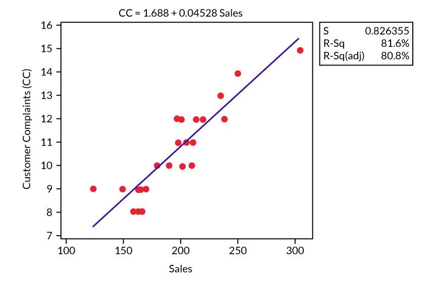
This model does nothing to explain cause. It simply offers evidence that there is a relationship between higher sales and higher numbers of complaints. If the manager were to use this simple linear regression to determine the cause of complaints, he might arrive at the logical conclusion to simply reduce sales in order to reduce complaints, which is ludicrous. Yet every practitioner can probably think of a time that a similar flaw was the entire basis of a misdirected project.
Based on the R2 value (percent of the variation explained by the model) of nearly 82 percent, there is evidence to support the expectation that customer complaints increase as sales increase, which would be beneficial for predictive purposes. But the manager’s original purpose was to try and explain the cause(s) of the complaints. Model 1 should be used as a predictive model within the range of values – but more about that later. The point? Practitioners or project teams must make sure they understand why they are using any regression technique.
2. Select Appropriate Variables
Back to the hypothetical data in the original table. Assume that the manager wants to know how much advertising influences sales and builds the following model (Figure 2).
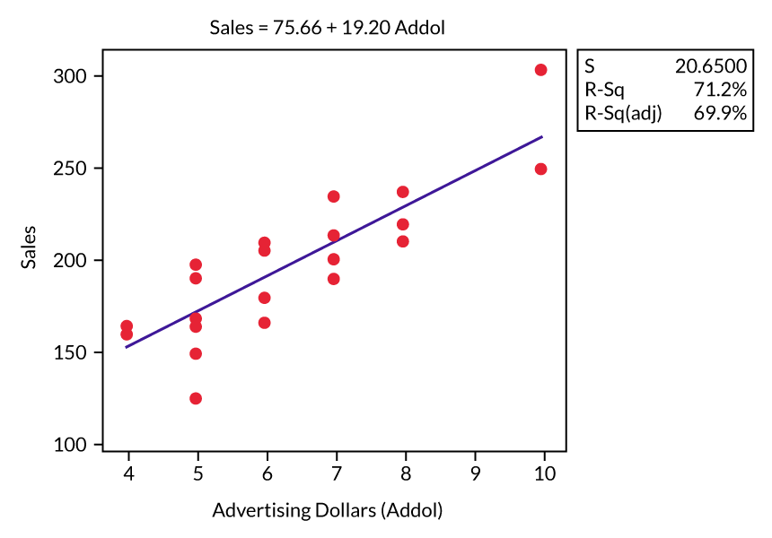
Model 2 seems to show some relationship between higher advertising dollars and increased sales. The question here is about the appropriateness of the variables used. Given the evidence (R2 value) the manager is correct if he asks, “Does my advertising budget influence sales?” and then tests the strength of the relationship with simple linear regression.
3. Straight – View Regression on a Plotted Line for Linearity
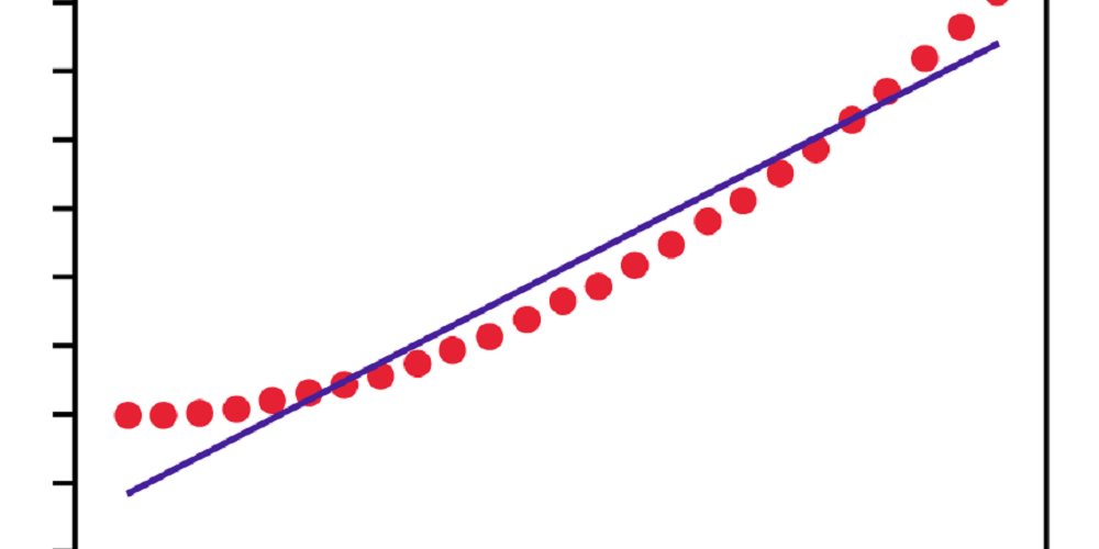
Models 1 and 2 are both reasonably linear. That is, both models are absent of curvilinear-patterned data. This is important. Suppose that the analysis produces a model that looks like Figure 3.
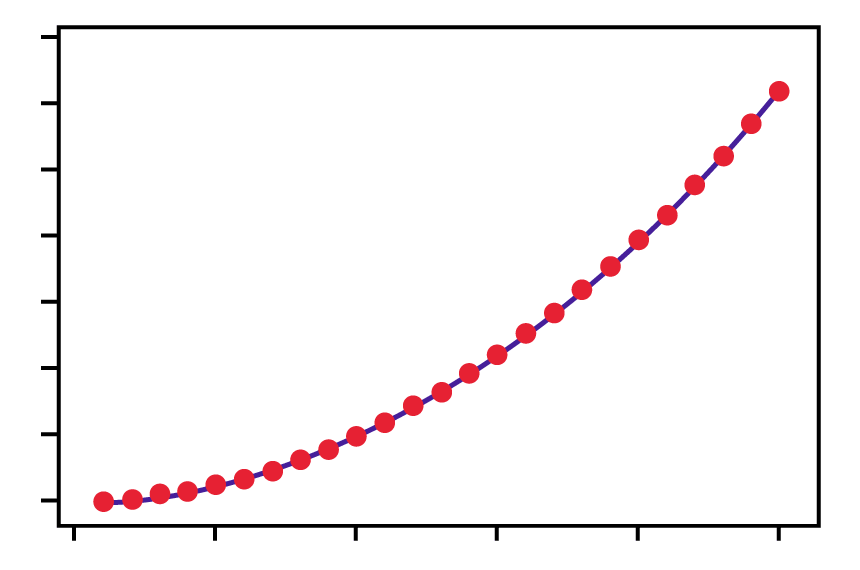
Model 3 shows a straight line through curved data. (This is only an example – real data rarely produces such a perfectly smooth curve.) In this case, simple linear regression is not reliable due to the residual pattern. A non-linear model would be more appropriate.
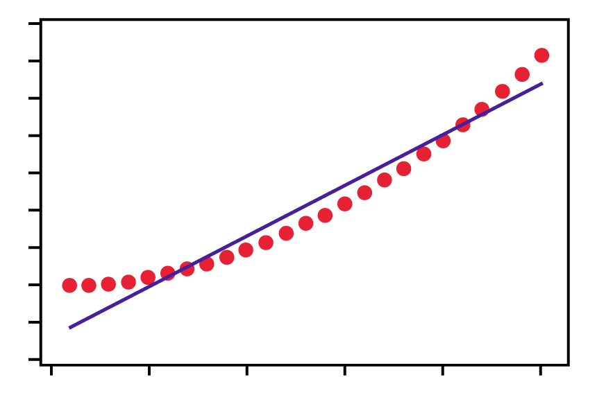
Figure 4 shows Model 4 which is the same data with a fitted line using a non-linear method. (It is important to validate a model. Use a residual and/or probability plot and look for normally distributed residuals.)
4. Sweep Away Outliers (When Appropriate)
Removing values from a data set can be controversial and wrong. However, there are times when removing outliers can be correct and beneficial. For an example, consider the imaginary manager and sales data from the table, and Model 5 in Figure 5 below.
Notice the two outliers? These come from points 22 and 23 from the table. From observing this model no evidence suggests that customer complaints are associated with sales (the R2 is low). Should these two outliers be removed? Will removing them change the data sets and be considered manipulating the model inappropriately?
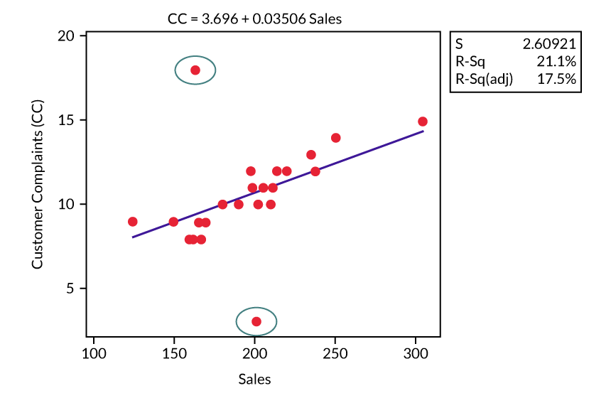
The answers depend on whether or not there is a good reason for the extreme values. For example, if the data in the months represented by points 22 and 23 were in error – assume that some of the complaints were recorded onto the next month’s report – the obvious correction would be to go back to see what the real values should be, then replace them.
The less obvious and more controversial matter concerning removing the outliers is whether or not there is sufficient reason to remove them without a “good” reason. Look at the next model (Figure 6) after completely removing the extreme values (points 22 and 23 from the table).
")
The impact of removing the two outliers had a significant effect on the model for predictive purposes (R2 of 82 percent). Ultimately, one must be comfortable with removing outliers and this decision should be based on sound reasoning. In this case, the manager would be missing an important message from his simple linear regression had the outliers not been removed: If complaints tend to be predictable and increase with sales, perhaps he should conduct surveys from these customers to identify a potential common cause of customer dissatisfaction.
5. Stay Away from Extrapolating Outside the Model
When simple linear regression is used for prediction, a response value is being obtained from the regression equation. For example, suppose the manager’s company has increased the sales force and advertising budget but nothing else has changed (no process improvement teams have begun to look into the root cause of the customer complaints). The manager wants to estimate (predict) how many complaints he will receive next month if the sales projection is accurate.
Based on Model 1, the regression equation was: Customer complaints = 1.688 + .04528 sales, which translates mathematically to: Y = 1.688 + .04528x
Suppose that sales are expected to be near $300,000. Since sales represent the x variable, the manager calculates complaints at: .04528 (300) + 1.688 = 15.27. Of course, it is impossible to have a fraction of a complaint so the manager could expect about 15 complaints in total. This lines up nicely with data from the table, at month 11 where sales were at $304,000 with 15 complaints.
What the managers did was interpolate, that is, he predicted a response within the model for a represented value. The x variables (sales) range from $125,000 to $304,000. But what if he were expecting sales at $400,000? Could he calculate a Y value at that level? Sure he could, although the experts generally warn against this and consider extrapolation more like guessing. In practice, many analysts extrapolate within reasonable bounds. (The issue is deciding what “reasonable” is.)
Conclusion: More Accurate Assessments
With more people becoming familiar with statistical techniques, and statistical software making regression analyses easily accessible, it is important to ensure that people are relying on usable regression models. That is why a reasonably easy way to assess simple linear regression analysis is needed – thus, allowing for more accurate predictions and measurement assessment.